Show the code
library(tidyverse)
library(mrgsolve)
library(gridExtra)

theme_set(theme_bw())
options(warn = -1)Visual predictive checks (VPCs) are frequently used for model evaluations in pharmacometric analyses. Recently, several engaging discussions on VPC fundamentals emerged during ECP8500 Advanced Pharmacometrics (aka. Pharmacometrics Coffee Break), which motivated the creation of this blog.
In this blog, we walk through the step-by-step process of constructing a VPC, to visually assess the predictive performance of a model by comparing simulated predictions against observed data.
Disclaimer: This blog is intended solely for educational purposes, and aim to illustrate, step-by-step, why VPC is needed and how VPC can be created without using packaged VPC functions. In practice, most of the procedures described here can be easily implemented using well-developed software tools, such as R packages vpc and tidyvpc, or similar functionality in other programs.
All data and model in this blog are synthetic and are included purely for demonstration purposes.
R packages (tidyverse, mrgsolve, gridExtra) are needed to execute the code in this blog.
library(tidyverse)
library(mrgsolve)
library(gridExtra)
theme_set(theme_bw())
options(warn = -1)A few helper functions were created to save some repetitive codes.
# Functions to plot raw PK (conc-time) profiles
raw_pk_plot <- function(df, .x=NTIME, .y=DV, .group=ID, .facet=DOSE,
                   logy=TRUE){
  p <- df %>% ggplot(aes(x={{.x}}, y={{.y}}, group={{.group}}))+
    geom_point()+geom_line(alpha=0.2)+
    facet_grid(rows=vars({{.facet}}), labeller=label_both)

  if(logy) p <- p + scale_y_log10()

  return(p)
}

# Functions to make summary PK profiles
summ_pk_plot <- function(df, .x=NTIME, .y=DV, .facet=DOSE,
                     logy=TRUE, show_obs=FALSE){
  dat <- df %>% group_by({{.x}}, {{.facet}}) %>%
    summarise(
      as_tibble_row(
        quantile({{.y}}, c(0.025, 0.500, 0.975),na.rm = TRUE),
        .name_repair= ~ c("lo", "mi", "hi")
      ),
      .groups = "drop")

  p <- dat %>% ggplot(aes(x={{.x}}))+
    geom_line(aes(y=mi))+
    geom_ribbon(aes(ymin=lo, ymax=hi), alpha=0.25)+
    facet_grid(vars({{.facet}}), labeller=label_both)+
    ylab("")

  if(show_obs) p <- p + geom_point(data=df, aes(x={{.x}}, y=DV))
  if(logy) p <- p + scale_y_log10()
  return(p)
}

# Functions to. ake VPC plots
vpcplot <- function(obs_df, sim_df,
                    .x=NTIME, .yobs=DV, .ysim=Y, .facet=DOSE,
                    .color=NULL, .xlab=NULL, .ylab=NULL,
                    percentile=c(0.10, 0.50, 0.90),
                    prob=c(0.10, 0.50, 0.90),
                    logy=TRUE, show_obs=FALSE, bins=NULL,
                    pcvpc=FALSE){


  # Assign ticks, calculate middles for plotting
  if (is.null(bins)) {
    ticks <- NULL
    mids  <- NULL
  } else {
    bins <- sort(unique(as.numeric(bins)))
    ticks <- cut(bins, breaks = bins)[-1]
    mids  <- (bins[-1] + bins[-length(bins)]) / 2 # Calculate midpoints for plotting
  }

  if (is.null(ticks)){
    obs_df <- obs_df %>% mutate(.bin = {{.x}},.x_plot = {{.x}})
    sim_df <- sim_df %>% mutate(.bin = {{.x}},.x_plot = {{.x}})
  }else{
    obs_df <- obs_df %>% mutate(
      .bin = cut({{.x}}, breaks = bins, include.lowest = TRUE, right = TRUE),
      .x_plot = mids[as.integer(.bin)])
    sim_df <- sim_df %>% mutate(
      .bin = cut({{.x}}, breaks = bins, include.lowest = TRUE, right = TRUE),
      .x_plot = mids[as.integer(.bin)])
  }

  # Summarise observed percentiles
   obs <- obs_df %>% group_by(.bin, .x_plot, {{.facet}}) %>%
      summarise(
        as_tibble_row(
          quantile({{.yobs}}, percentile,na.rm = TRUE),
          .name_repair= ~ c("lo", "mi", "hi")
        ),
        .groups = "drop")

  # Summarise simulated percentiles
  sim <- sim_df %>% group_by(.bin, .x_plot, {{.facet}}, IREP) %>%
    summarise(
      as_tibble_row(
        quantile({{.ysim}}, percentile,na.rm = TRUE),
        .name_repair= ~ c("lo", "mi", "hi")
      ),
      .groups = "drop")

  # Prediction correction
  if(pcvpc){
    # stopifnot("PRED" %in% names(sim_df))

    obs <- obs_df %>% mutate(.yobs = {{.yobs}}/PRED) %>%
      group_by(.bin, .x_plot, {{.facet}}) %>%
      mutate(pred_bin = median(PRED)) %>%
      mutate(.yobs = .yobs*pred_bin) %>%
      summarise(
        as_tibble_row(
          quantile(.yobs, percentile,na.rm = TRUE),
          .name_repair= ~ c("lo", "mi", "hi")
        ),
        .groups = "drop")

    sim <- sim_df %>% mutate(.ysim = {{.ysim}}/PRED) %>%
      group_by(.bin, .x_plot, {{.facet}}, IREP) %>%
      mutate(pred_bin = median(PRED)) %>%
      mutate(.ysim = .ysim*pred_bin) %>%
      summarise(
        as_tibble_row(
          quantile(.ysim, percentile,na.rm = TRUE),
          .name_repair= ~ c("lo", "mi", "hi")
        ),
        .groups = "drop")
  }

  # Summarise prediction intervals of simulated percentiles
  sim <- sim %>% group_by(.bin, .x_plot, {{.facet}}) %>%
    summarise(
      across(c("lo", "mi", "hi"),
             ~ list(setNames(
               quantile(.x, prob, na.rm = TRUE),
               c("lo", "mi", "hi")
             ))),
      .groups = "drop"
    ) %>%
    # widen each list-column (one per Y) into 3 numeric columns
    unnest_wider(c("lo", "mi", "hi"), names_sep = "_")

  p <- ggplot()+
    geom_line(data=obs, aes(x=.x_plot, y=lo), linetype=2)+
    geom_line(data=obs, aes(x=.x_plot, y=mi), linetype=1)+
    geom_line(data=obs, aes(x=.x_plot, y=hi), linetype=2)+
    geom_ribbon(data=sim, aes(x=.x_plot, ymin=lo_lo, ymax=lo_hi), alpha=0.25, fill="#ffcc33")+
    geom_ribbon(data=sim, aes(x=.x_plot, ymin=mi_lo, ymax=mi_hi), alpha=0.25, fill="#7A0019")+
    geom_ribbon(data=sim, aes(x=.x_plot, ymin=hi_lo, ymax=hi_hi), alpha=0.25, fill="#ffcc33")+
    facet_grid(vars({{.facet}}), labeller=label_both)

  if(!is.null(xlab)) p <- p+xlab(.xlab)
  if(!is.null(ylab)) p <- p+ylab(.ylab)

  if(show_obs) p <- p + geom_point(data=obs_df, aes(x={{.x}}, y={{.yobs}}, color={{.color}}))

  if(pcvpc&show_obs){
    obs_df2 <- obs_df %>% mutate(.yobs = {{.yobs}}/PRED) %>%
      group_by(.bin, .x_plot, {{.facet}}) %>%
      mutate(pred_bin = median(PRED)) %>%
      mutate(.yobs = .yobs*pred_bin)
    p <- p + geom_point(data=obs_df2, aes(x={{.x}}, y=.yobs, color={{.color}}))
  }

  if(!is.null(bins)) p <- p + scale_x_continuous(
    limits = range(bins),
    expand = expansion(mult = c(0, 0.02)),
    sec.axis = dup_axis(
      name   = NULL,
      breaks = bins,           # tick positions on top
      labels = rep("", length(bins))  # no labels, ticks only
    )) + theme(
      axis.ticks.x.top  = element_line(),
      axis.ticks.length.x.top = unit(5, "pt")
    )

  if(logy) p <- p + scale_y_log10()

  return(p)
}An example PK model was created for the purpose of illustration:
A one-compartment PK model, with zero- and first-order absorptions (KA and D1) and first-order elimination.
Body weight was added as a covariate on clearance (CL) and volume (V) using standard allometric scaling with exponents of 0.75 and 1.
Sex, age and albumin were added as covariates on CL.
Interindividual variabilities were added on CL, V and D1, with full omega matrix specified.
Proportional error model was assumed to describe residual errors.
code <- '
  [ prob ]
    One-compartmental model + 0 and 1st order abs and 1st order elim
    Allometric scaling on CL and V patrameters
    Covariate-effects (SEX, AGE, ALB) on CL
    Proportional error model
    This model requires mrgsolve >= 1.0.3

  [ cmt ] depot cent

  [ input ]
    WT  = 70
    SEX = 1
    AGE = 35
    ALB = 4.5

  [ theta ]
    1.5    //  1 CL (L/hr) - 3.5
    5.0    //  2 V  (L) - 60
    0.5    //  3 KA (1/hr) - 1.5
    0.8    //  4 D1 (/hr) - 1.5
    0.7    //  5 SEX~CL (fractional multiplier)
    0.5    //  6 AGE~CL (exponent)
    0.2    //  7 ALB~CL (exponent)
    0.75   //  8 WT~CL (exponent)
    1.0    //  9 WT~CL (exponent)

  [ omega ] @correlation
    0.15             // ETA(CL)
    0.50 0.15        // ETA(V)
    0.10 0.20 0.1    // ETA(D1)

  [ sigma ]
    0.15              // Prop

    [ pk ]
    // Typical values of PK parameters
    double TVCL   = THETA(1);
    double TVV    = THETA(2);
    double TVKA   = THETA(3);
    double TVD1   = THETA(4);

    // PK covariates
    double CL_SEX = pow(THETA(5)  , SEX-1   );
    double CL_AGE = pow((AGE/35.0), THETA(6));
    double CL_ALB = pow((ALB/4.5) , THETA(7));
    double CL_WT  = pow((WT/70)   , THETA(8));
    double V_WT   = pow((WT/70)   , THETA(9));

    double CLCOV = CL_AGE*CL_WT;
    double VCOV  = V_WT;

    // PK parameters
    double CL = TVCL*CLCOV*exp(ETA(1));
    double V  = TVV*VCOV*exp(ETA(2));
    double KA = TVKA;
    double D1 = TVD1*exp(ETA(3));

    double S2 = V;

    D_depot = D1;

  [ ode ]
    dxdt_depot = -KA*depot;
    dxdt_cent = KA*depot - (CL/V)*cent;

  [ error ]
    double IPRED = cent/S2;
    double Y = IPRED * (1+EPS(1));

  [ capture ] CL V IPRED Y
  '
Let’s load the above PK model in R.
# Load model
mod <- mcode("example", code)
Building example ... done.Let’s also load the data in NONMEM format, which have both doses, observations and covariates.
data <- structure(list(C = c(".", ".", ".", ".", ".", ".", ".", ".",
".", ".", ".", ".", ".", ".", ".", ".", ".", ".", ".", ".", ".",
".", ".", ".", ".", ".", ".", ".", ".", ".", ".", ".", ".", ".",
".", ".", ".", ".", ".", ".", ".", ".", ".", ".", ".", ".", ".",
".", ".", ".", ".", ".", ".", ".", ".", ".", ".", ".", ".", ".",
".", ".", ".", ".", ".", ".", ".", ".", ".", ".", ".", ".", ".",
".", ".", ".", ".", ".", ".", ".", ".", ".", ".", ".", ".", ".",
".", ".", ".", ".", ".", ".", ".", ".", ".", ".", ".", ".", ".",
".", ".", ".", ".", ".", ".", ".", ".", ".", ".", ".", ".", ".",
".", ".", ".", ".", ".", ".", ".", ".", ".", ".", ".", ".", ".",
".", ".", ".", ".", ".", ".", ".", ".", ".", ".", ".", ".", ".",
".", ".", ".", ".", ".", ".", ".", ".", ".", ".", ".", ".", ".",
".", ".", ".", ".", ".", ".", ".", ".", ".", ".", ".", ".", ".",
".", ".", ".", ".", ".", ".", ".", ".", ".", ".", ".", ".", ".",
".", ".", ".", ".", ".", ".", ".", ".", ".", ".", ".", ".", ".",
".", ".", ".", ".", ".", ".", ".", ".", ".", ".", ".", ".", ".",
".", ".", ".", ".", ".", ".", ".", ".", ".", ".", ".", ".", ".",
".", ".", ".", ".", ".", ".", ".", ".", ".", ".", ".", ".", ".",
".", ".", ".", ".", ".", ".", ".", ".", ".", ".", ".", ".", ".",
".", ".", ".", ".", ".", ".", ".", ".", ".", ".", ".", ".", ".",
".", ".", ".", ".", ".", ".", ".", ".", ".", ".", ".", ".", ".",
".", ".", ".", ".", ".", ".", ".", ".", ".", ".", ".", ".", ".",
".", ".", ".", ".", ".", ".", ".", ".", ".", ".", ".", ".", ".",
".", ".", ".", ".", ".", ".", ".", ".", ".", ".", ".", ".", ".",
".", ".", ".", ".", ".", ".", ".", ".", ".", ".", ".", ".", ".",
".", ".", ".", ".", ".", ".", ".", ".", ".", ".", ".", ".", ".",
".", ".", ".", ".", ".", ".", ".", ".", ".", ".", ".", ".", ".",
".", ".", ".", ".", ".", ".", ".", ".", ".", ".", ".", ".", ".",
".", ".", ".", ".", ".", ".", ".", ".", ".", ".", ".", ".", ".",
".", ".", ".", ".", ".", ".", ".", ".", ".", ".", ".", ".", ".",
".", ".", ".", ".", ".", ".", ".", ".", ".", ".", ".", ".", ".",
".", ".", ".", ".", ".", ".", ".", ".", ".", ".", ".", ".", ".",
".", ".", ".", ".", ".", ".", ".", ".", ".", ".", ".", ".", ".",
".", ".", ".", ".", ".", ".", ".", ".", ".", ".", ".", ".", ".",
".", ".", ".", ".", ".", ".", ".", ".", ".", ".", ".", ".", ".",
".", ".", ".", ".", ".", ".", ".", ".", ".", ".", ".", ".", ".",
".", ".", ".", ".", ".", ".", ".", ".", ".", ".", ".", ".", ".",
".", ".", ".", ".", ".", ".", ".", ".", ".", ".", ".", ".", ".",
".", ".", ".", ".", ".", ".", ".", ".", ".", ".", ".", ".", ".",
".", ".", ".", ".", ".", ".", ".", ".", ".", ".", ".", ".", ".",
".", ".", ".", ".", ".", ".", ".", ".", ".", ".", ".", ".", ".",
".", ".", ".", ".", ".", ".", ".", ".", ".", ".", ".", ".", ".",
".", ".", ".", ".", ".", ".", ".", ".", ".", ".", ".", ".", ".",
".", ".", ".", ".", ".", ".", ".", ".", ".", ".", ".", ".", ".",
".", ".", ".", ".", ".", ".", ".", ".", ".", ".", ".", ".", ".",
".", ".", ".", ".", ".", ".", ".", ".", ".", ".", ".", ".", ".",
".", ".", ".", ".", ".", ".", ".", ".", ".", ".", ".", ".", ".",
".", ".", ".", ".", ".", ".", ".", ".", ".", ".", ".", ".", ".",
".", ".", ".", ".", ".", ".", ".", ".", ".", ".", ".", ".", ".",
".", ".", ".", ".", ".", ".", ".", ".", ".", ".", ".", ".", ".",
".", ".", ".", ".", ".", "."), NUM = 1:651, ID = c(51L, 51L,
51L, 51L, 51L, 51L, 52L, 52L, 52L, 52L, 52L, 52L, 53L, 53L, 53L,
53L, 53L, 53L, 53L, 54L, 54L, 54L, 54L, 54L, 55L, 55L, 55L, 55L,
55L, 55L, 56L, 56L, 56L, 56L, 56L, 56L, 56L, 57L, 57L, 57L, 57L,
57L, 57L, 58L, 58L, 58L, 58L, 58L, 58L, 59L, 59L, 59L, 59L, 59L,
59L, 60L, 60L, 60L, 60L, 60L, 60L, 61L, 61L, 61L, 61L, 61L, 62L,
62L, 62L, 62L, 62L, 62L, 62L, 63L, 63L, 63L, 63L, 63L, 63L, 64L,
64L, 64L, 64L, 64L, 64L, 64L, 65L, 65L, 65L, 65L, 65L, 65L, 66L,
66L, 66L, 66L, 66L, 66L, 67L, 67L, 67L, 67L, 67L, 67L, 68L, 68L,
68L, 68L, 68L, 69L, 69L, 69L, 69L, 69L, 70L, 70L, 70L, 70L, 70L,
70L, 71L, 71L, 71L, 71L, 71L, 72L, 72L, 72L, 72L, 72L, 72L, 72L,
73L, 73L, 73L, 73L, 73L, 74L, 74L, 74L, 74L, 74L, 75L, 75L, 75L,
75L, 75L, 75L, 76L, 76L, 76L, 76L, 76L, 77L, 77L, 77L, 77L, 77L,
77L, 77L, 78L, 78L, 78L, 78L, 78L, 78L, 79L, 79L, 79L, 79L, 79L,
80L, 80L, 80L, 80L, 80L, 80L, 80L, 81L, 81L, 81L, 81L, 81L, 82L,
82L, 82L, 82L, 82L, 83L, 83L, 83L, 83L, 83L, 83L, 83L, 84L, 84L,
84L, 84L, 84L, 85L, 85L, 85L, 85L, 85L, 86L, 86L, 86L, 86L, 86L,
86L, 86L, 87L, 87L, 87L, 87L, 87L, 88L, 88L, 88L, 88L, 88L, 88L,
89L, 89L, 89L, 89L, 89L, 89L, 90L, 90L, 90L, 90L, 90L, 90L, 91L,
91L, 91L, 91L, 91L, 91L, 91L, 92L, 92L, 92L, 92L, 92L, 92L, 92L,
93L, 93L, 93L, 93L, 93L, 93L, 93L, 94L, 94L, 94L, 94L, 94L, 94L,
95L, 95L, 95L, 95L, 95L, 95L, 95L, 96L, 96L, 96L, 96L, 96L, 96L,
97L, 97L, 97L, 97L, 97L, 97L, 98L, 98L, 98L, 98L, 98L, 98L, 98L,
99L, 99L, 99L, 99L, 99L, 99L, 99L, 100L, 100L, 100L, 100L, 100L,
100L, 100L, 101L, 101L, 101L, 102L, 102L, 103L, 103L, 103L, 103L,
104L, 104L, 104L, 104L, 105L, 105L, 105L, 105L, 106L, 106L, 106L,
107L, 107L, 107L, 108L, 108L, 108L, 108L, 109L, 109L, 109L, 109L,
110L, 110L, 110L, 110L, 111L, 111L, 111L, 112L, 112L, 112L, 112L,
113L, 113L, 113L, 113L, 114L, 114L, 114L, 114L, 115L, 115L, 115L,
116L, 116L, 116L, 116L, 117L, 117L, 117L, 117L, 118L, 118L, 118L,
118L, 119L, 119L, 119L, 119L, 120L, 120L, 120L, 120L, 121L, 121L,
121L, 121L, 122L, 122L, 122L, 123L, 123L, 123L, 123L, 124L, 124L,
124L, 124L, 125L, 125L, 125L, 125L, 126L, 126L, 126L, 126L, 127L,
127L, 127L, 128L, 128L, 128L, 129L, 129L, 129L, 129L, 130L, 130L,
130L, 131L, 131L, 131L, 132L, 132L, 132L, 132L, 133L, 133L, 133L,
134L, 134L, 134L, 134L, 135L, 135L, 135L, 135L, 136L, 136L, 136L,
136L, 137L, 137L, 137L, 137L, 138L, 138L, 138L, 138L, 139L, 139L,
139L, 139L, 140L, 140L, 140L, 141L, 141L, 141L, 142L, 142L, 142L,
143L, 143L, 143L, 143L, 144L, 144L, 144L, 144L, 145L, 145L, 145L,
146L, 146L, 146L, 146L, 147L, 147L, 147L, 148L, 148L, 148L, 149L,
149L, 149L, 149L, 150L, 150L, 150L, 150L, 151L, 151L, 151L, 152L,
152L, 152L, 152L, 153L, 153L, 153L, 153L, 154L, 154L, 154L, 155L,
155L, 155L, 155L, 156L, 156L, 156L, 156L, 157L, 157L, 157L, 158L,
158L, 159L, 159L, 159L, 159L, 160L, 161L, 161L, 161L, 162L, 162L,
162L, 162L, 163L, 163L, 163L, 164L, 164L, 165L, 165L, 165L, 166L,
166L, 166L, 166L, 167L, 167L, 168L, 168L, 168L, 168L, 169L, 169L,
169L, 170L, 170L, 170L, 170L, 171L, 171L, 171L, 172L, 172L, 173L,
173L, 173L, 173L, 174L, 174L, 174L, 174L, 175L, 175L, 175L, 175L,
176L, 176L, 176L, 177L, 177L, 177L, 178L, 178L, 178L, 178L, 179L,
179L, 179L, 179L, 180L, 180L, 180L, 180L, 181L, 181L, 181L, 182L,
182L, 182L, 182L, 183L, 183L, 183L, 183L, 184L, 184L, 184L, 184L,
185L, 185L, 186L, 186L, 186L, 187L, 187L, 188L, 188L, 188L, 188L,
189L, 189L, 189L, 189L, 190L, 190L, 190L, 191L, 191L, 191L, 192L,
192L, 192L, 192L, 193L, 193L, 193L, 193L, 194L, 194L, 194L, 194L,
195L, 195L, 195L, 196L, 196L, 196L, 196L, 197L, 197L, 197L, 198L,
198L, 198L, 198L, 199L, 199L, 199L, 200L, 200L, 200L, 200L),
    TIME = c(0, 120.09, 121.04, 124.07, 128.24, 139.22, 0, 120.1,
    120.23, 120.96, 127.76, 140.79, 0, 120.09, 120.23, 121.08,
    124.11, 128.01, 138.3, 0, 120.09, 120.98, 124.22, 140.45,
    0, 120.1, 120.24, 121.1, 124.09, 138.02, 0, 120.09, 120.26,
    121, 124.26, 128.06, 140.52, 0, 120.11, 120.25, 120.93, 123.94,
    127.64, 0, 120.1, 120.25, 124.05, 128.11, 138.18, 0, 120.09,
    120.23, 123.74, 128.29, 141.57, 0, 120.09, 120.26, 121.01,
    123.68, 127.55, 0, 120.09, 120.26, 128.14, 138.9, 0, 120.11,
    120.23, 121.07, 123.82, 128.41, 139.92, 0, 120.1, 120.24,
    124.37, 128.46, 138.33, 0, 120.1, 120.27, 120.94, 124.04,
    127.7, 140.66, 0, 120.1, 121.06, 123.65, 127.52, 139.82,
    0, 120.09, 120.24, 123.99, 128.48, 139.13, 0, 120.1, 120.27,
    121.09, 123.88, 138.5, 0, 120.1, 120.99, 123.84, 127.32,
    0, 120.09, 121.09, 128.53, 139.57, 0, 120.1, 120.24, 121.02,
    128.75, 141.85, 0, 120.1, 120.23, 123.89, 128.06, 0, 120.09,
    120.24, 121, 124.08, 128.43, 140.56, 0, 120.26, 124.29, 128.6,
    139.6, 0, 120.09, 120.23, 120.96, 123.67, 0, 120.1, 120.25,
    124.24, 127.46, 139.65, 0, 120.11, 121.01, 123.74, 141.26,
    0, 120.09, 120.23, 120.97, 123.75, 128.49, 139.87, 0, 120.09,
    120.25, 123.78, 127.83, 140.4, 0, 120.11, 120.97, 128.25,
    138.1, 0, 120.1, 120.24, 120.91, 123.96, 127.82, 138.24,
    0, 120.25, 121.1, 128.27, 141.92, 0, 120.11, 120.26, 121.07,
    127.45, 0, 120.1, 120.25, 121.09, 123.75, 128.24, 139.52,
    0, 120.11, 120.91, 128.08, 140.79, 0, 120.1, 120.26, 121.09,
    124.22, 0, 120.09, 120.23, 121.01, 123.7, 127.61, 138.07,
    0, 120.27, 121.08, 127.67, 140.02, 0, 120.09, 120.24, 121.08,
    123.84, 141.29, 0, 120.1, 120.23, 120.99, 128.65, 140.68,
    0, 120.1, 120.23, 121.09, 124.02, 138.3, 0, 120.1, 120.23,
    120.93, 124.02, 127.45, 141.36, 0, 120.11, 120.26, 121.05,
    124.31, 127.98, 141.96, 0, 120.11, 120.26, 120.91, 123.89,
    127.82, 140.5, 0, 120.23, 121.1, 124.12, 127.8, 141.43, 0,
    120.11, 120.24, 121.07, 123.77, 128.66, 141.52, 0, 120.25,
    120.92, 124.02, 127.45, 138.83, 0, 120.1, 120.27, 120.92,
    124.37, 138.8, 0, 120.11, 120.24, 121.03, 123.95, 128.15,
    140.21, 0, 120.1, 120.24, 121.07, 124.09, 128.19, 141.91,
    0, 120.1, 120.23, 121.05, 124.36, 127.84, 141.04, 0, 124.2,
    141.7, 0, 121, 0, 121, 123.9, 139.41, 0, 120.93, 124.31,
    138.11, 0, 121.08, 123.98, 141.41, 0, 121.09, 124.29, 0,
    121.02, 139.94, 0, 121.04, 123.77, 139.04, 0, 121, 124.22,
    141.01, 0, 120.99, 124.28, 140.16, 0, 124.15, 140.94, 0,
    121.02, 124.29, 139.83, 0, 121.04, 123.75, 141.8, 0, 120.94,
    124.3, 141.93, 0, 120.92, 124.07, 0, 120.98, 123.95, 141.4,
    0, 121.02, 123.98, 141.38, 0, 121, 124.24, 138.44, 0, 121.05,
    124.39, 141.45, 0, 121.09, 124.3, 141.78, 0, 120.92, 124.07,
    139.09, 0, 123.68, 140, 0, 120.95, 123.85, 141.17, 0, 120.93,
    124.34, 140.93, 0, 120.9, 124.32, 138.21, 0, 120.97, 123.64,
    138.17, 0, 121.02, 124.27, 0, 121.04, 139.1, 0, 121.09, 123.88,
    141.05, 0, 121.08, 123.75, 0, 121, 123.7, 0, 121.03, 124.26,
    139.4, 0, 124.22, 141.48, 0, 120.98, 123.67, 141.42, 0, 121.01,
    123.77, 138.41, 0, 121.03, 124.18, 139.27, 0, 120.91, 124.39,
    140.33, 0, 121.04, 123.99, 138.71, 0, 121.1, 124.06, 138.6,
    0, 123.61, 141.52, 0, 120.94, 124.37, 0, 120.98, 124.11,
    0, 120.94, 124.23, 141.72, 0, 121.1, 124.38, 140.72, 0, 123.68,
    139.71, 0, 121, 124.04, 140.57, 0, 120.96, 139.93, 0, 124.34,
    138.53, 0, 120.94, 123.98, 139.86, 0, 121.04, 124.06, 139.6,
    0, 121.05, 140.17, 0, 121.06, 124.18, 141.19, 0, 120.96,
    123.65, 140.24, 0, 124.34, 140.34, 0, 120.98, 124.21, 140.87,
    0, 121.03, 123.8, 139.03, 0, 124.1, 139.24, 0, 138.37, 0,
    121.06, 123.89, 141.52, 0, 0, 124.14, 139.94, 0, 120.95,
    124.22, 140.85, 0, 121.04, 123.86, 0, 123.93, 0, 120.91,
    124.17, 0, 120.91, 123.98, 141.35, 0, 140.09, 0, 121.06,
    124.21, 141.15, 0, 124.14, 139.03, 0, 120.96, 124.19, 139.74,
    0, 120.95, 123.69, 0, 120.98, 0, 121.01, 124.2, 140.82, 0,
    121.02, 123.82, 141.01, 0, 121.09, 124.17, 141.18, 0, 121.07,
    124.01, 0, 121.03, 124.1, 0, 120.99, 124.3, 141.68, 0, 120.95,
    124.27, 140.66, 0, 120.92, 123.81, 140.33, 0, 120.99, 124.22,
    0, 120.91, 124.35, 138.15, 0, 120.93, 124.07, 141.39, 0,
    121.05, 124.28, 139.89, 0, 139.48, 0, 123.78, 139.84, 0,
    140.48, 0, 121.08, 124.34, 140.09, 0, 121.07, 123.83, 138.28,
    0, 124.3, 140.92, 0, 120.96, 123.93, 0, 120.98, 123.78, 140.78,
    0, 121.03, 124.38, 138.67, 0, 120.97, 123.96, 141.15, 0,
    121, 123.8, 0, 121.03, 124.34, 140.29, 0, 121.08, 123.81,
    0, 121.07, 124.06, 139.77, 0, 123.99, 138.46, 0, 121.05,
    124.1, 139.26), NTIME = c(120.1, 120.1, 121, 124, 128, 140,
    120.1, 120.1, 120.25, 121, 128, 140, 120.1, 120.1, 120.25,
    121, 124, 128, 140, 120.1, 120.1, 121, 124, 140, 120.1, 120.1,
    120.25, 121, 124, 140, 120.1, 120.1, 120.25, 121, 124, 128,
    140, 120.1, 120.1, 120.25, 121, 124, 128, 120.1, 120.1, 120.25,
    124, 128, 140, 120.1, 120.1, 120.25, 124, 128, 140, 120.1,
    120.1, 120.25, 121, 124, 128, 120.1, 120.1, 120.25, 128,
    140, 120.1, 120.1, 120.25, 121, 124, 128, 140, 120.1, 120.1,
    120.25, 124, 128, 140, 120.1, 120.1, 120.25, 121, 124, 128,
    140, 120.1, 120.1, 121, 124, 128, 140, 120.1, 120.1, 120.25,
    124, 128, 140, 120.1, 120.1, 120.25, 121, 124, 140, 120.1,
    120.1, 121, 124, 128, 120.1, 120.1, 121, 128, 140, 120.1,
    120.1, 120.25, 121, 128, 140, 120.1, 120.1, 120.25, 124,
    128, 120.1, 120.1, 120.25, 121, 124, 128, 140, 120.1, 120.25,
    124, 128, 140, 120.1, 120.1, 120.25, 121, 124, 120.1, 120.1,
    120.25, 124, 128, 140, 120.1, 120.1, 121, 124, 140, 120.1,
    120.1, 120.25, 121, 124, 128, 140, 120.1, 120.1, 120.25,
    124, 128, 140, 120.1, 120.1, 121, 128, 140, 120.1, 120.1,
    120.25, 121, 124, 128, 140, 120.1, 120.25, 121, 128, 140,
    120.1, 120.1, 120.25, 121, 128, 120.1, 120.1, 120.25, 121,
    124, 128, 140, 120.1, 120.1, 121, 128, 140, 120.1, 120.1,
    120.25, 121, 124, 120.1, 120.1, 120.25, 121, 124, 128, 140,
    120.1, 120.25, 121, 128, 140, 120.1, 120.1, 120.25, 121,
    124, 140, 120.1, 120.1, 120.25, 121, 128, 140, 120.1, 120.1,
    120.25, 121, 124, 140, 120.1, 120.1, 120.25, 121, 124, 128,
    140, 120.1, 120.1, 120.25, 121, 124, 128, 140, 120.1, 120.1,
    120.25, 121, 124, 128, 140, 120.1, 120.25, 121, 124, 128,
    140, 120.1, 120.1, 120.25, 121, 124, 128, 140, 120.1, 120.25,
    121, 124, 128, 140, 120.1, 120.1, 120.25, 121, 124, 140,
    120.1, 120.1, 120.25, 121, 124, 128, 140, 120.1, 120.1, 120.25,
    121, 124, 128, 140, 120.1, 120.1, 120.25, 121, 124, 128,
    140, 120.1, 124, 140, 120.1, 121, 120.1, 121, 124, 140, 120.1,
    121, 124, 140, 120.1, 121, 124, 140, 120.1, 121, 124, 120.1,
    121, 140, 120.1, 121, 124, 140, 120.1, 121, 124, 140, 120.1,
    121, 124, 140, 120.1, 124, 140, 120.1, 121, 124, 140, 120.1,
    121, 124, 140, 120.1, 121, 124, 140, 120.1, 121, 124, 120.1,
    121, 124, 140, 120.1, 121, 124, 140, 120.1, 121, 124, 140,
    120.1, 121, 124, 140, 120.1, 121, 124, 140, 120.1, 121, 124,
    140, 120.1, 124, 140, 120.1, 121, 124, 140, 120.1, 121, 124,
    140, 120.1, 121, 124, 140, 120.1, 121, 124, 140, 120.1, 121,
    124, 120.1, 121, 140, 120.1, 121, 124, 140, 120.1, 121, 124,
    120.1, 121, 124, 120.1, 121, 124, 140, 120.1, 124, 140, 120.1,
    121, 124, 140, 120.1, 121, 124, 140, 120.1, 121, 124, 140,
    120.1, 121, 124, 140, 120.1, 121, 124, 140, 120.1, 121, 124,
    140, 120.1, 124, 140, 120.1, 121, 124, 120.1, 121, 124, 120.1,
    121, 124, 140, 120.1, 121, 124, 140, 120.1, 124, 140, 120.1,
    121, 124, 140, 120.1, 121, 140, 120.1, 124, 140, 120.1, 121,
    124, 140, 120.1, 121, 124, 140, 120.1, 121, 140, 120.1, 121,
    124, 140, 120.1, 121, 124, 140, 120.1, 124, 140, 120.1, 121,
    124, 140, 120.1, 121, 124, 140, 120.1, 124, 140, 120.1, 140,
    120.1, 121, 124, 140, 120.1, 120.1, 124, 140, 120.1, 121,
    124, 140, 120.1, 121, 124, 120.1, 124, 120.1, 121, 124, 120.1,
    121, 124, 140, 120.1, 140, 120.1, 121, 124, 140, 120.1, 124,
    140, 120.1, 121, 124, 140, 120.1, 121, 124, 120.1, 121, 120.1,
    121, 124, 140, 120.1, 121, 124, 140, 120.1, 121, 124, 140,
    120.1, 121, 124, 120.1, 121, 124, 120.1, 121, 124, 140, 120.1,
    121, 124, 140, 120.1, 121, 124, 140, 120.1, 121, 124, 120.1,
    121, 124, 140, 120.1, 121, 124, 140, 120.1, 121, 124, 140,
    120.1, 140, 120.1, 124, 140, 120.1, 140, 120.1, 121, 124,
    140, 120.1, 121, 124, 140, 120.1, 124, 140, 120.1, 121, 124,
    120.1, 121, 124, 140, 120.1, 121, 124, 140, 120.1, 121, 124,
    140, 120.1, 121, 124, 120.1, 121, 124, 140, 120.1, 121, 124,
    120.1, 121, 124, 140, 120.1, 124, 140, 120.1, 121, 124, 140
    ), TAD = c(0, 0.09, 1.04, 4.07, 8.24, 19.22, 0, 0.1, 0.23,
    0.96, 7.76, 20.79, 0, 0.09, 0.23, 1.08, 4.11, 8.01, 18.3,
    0, 0.09, 0.98, 4.22, 20.45, 0, 0.1, 0.24, 1.1, 4.09, 18.02,
    0, 0.09, 0.26, 1, 4.26, 8.06, 20.52, 0, 0.11, 0.25, 0.93,
    3.94, 7.64, 0, 0.1, 0.25, 4.05, 8.11, 18.18, 0, 0.09, 0.23,
    3.74, 8.29, 21.57, 0, 0.09, 0.26, 1.01, 3.68, 7.55, 0, 0.09,
    0.26, 8.14, 18.9, 0, 0.11, 0.23, 1.07, 3.82, 8.41, 19.92,
    0, 0.1, 0.24, 4.37, 8.46, 18.33, 0, 0.1, 0.27, 0.94, 4.04,
    7.7, 20.66, 0, 0.1, 1.06, 3.65, 7.52, 19.82, 0, 0.09, 0.24,
    3.99, 8.48, 19.13, 0, 0.1, 0.27, 1.09, 3.88, 18.5, 0, 0.1,
    0.99, 3.84, 7.32, 0, 0.09, 1.09, 8.53, 19.57, 0, 0.1, 0.24,
    1.02, 8.75, 21.85, 0, 0.1, 0.23, 3.89, 8.06, 0, 0.09, 0.24,
    1, 4.08, 8.43, 20.56, 0, 0.26, 4.29, 8.6, 19.6, 0, 0.09,
    0.23, 0.96, 3.67, 0, 0.1, 0.25, 4.24, 7.46, 19.65, 0, 0.11,
    1.01, 3.74, 21.26, 0, 0.09, 0.23, 0.97, 3.75, 8.49, 19.87,
    0, 0.09, 0.25, 3.78, 7.83, 20.4, 0, 0.11, 0.97, 8.25, 18.1,
    0, 0.1, 0.24, 0.91, 3.96, 7.82, 18.24, 0, 0.25, 1.1, 8.27,
    21.92, 0, 0.11, 0.26, 1.07, 7.45, 0, 0.1, 0.25, 1.09, 3.75,
    8.24, 19.52, 0, 0.11, 0.91, 8.08, 20.79, 0, 0.1, 0.26, 1.09,
    4.22, 0, 0.09, 0.23, 1.01, 3.7, 7.61, 18.07, 0, 0.27, 1.08,
    7.67, 20.02, 0, 0.09, 0.24, 1.08, 3.84, 21.29, 0, 0.1, 0.23,
    0.99, 8.65, 20.68, 0, 0.1, 0.23, 1.09, 4.02, 18.3, 0, 0.1,
    0.23, 0.93, 4.02, 7.45, 21.36, 0, 0.11, 0.26, 1.05, 4.31,
    7.98, 21.96, 0, 0.11, 0.26, 0.91, 3.89, 7.82, 20.5, 0, 0.23,
    1.1, 4.12, 7.8, 21.43, 0, 0.11, 0.24, 1.07, 3.77, 8.66, 21.52,
    0, 0.25, 0.92, 4.02, 7.45, 18.83, 0, 0.1, 0.27, 0.92, 4.37,
    18.8, 0, 0.11, 0.24, 1.03, 3.95, 8.15, 20.21, 0, 0.1, 0.24,
    1.07, 4.09, 8.19, 21.91, 0, 0.1, 0.23, 1.05, 4.36, 7.84,
    21.04, 0, 4.2, 21.7, 0, 1, 0, 1, 3.9, 19.41, 0, 0.93, 4.31,
    18.11, 0, 1.08, 3.98, 21.41, 0, 1.09, 4.29, 0, 1.02, 19.94,
    0, 1.04, 3.77, 19.04, 0, 1, 4.22, 21.01, 0, 0.99, 4.28, 20.16,
    0, 4.15, 20.94, 0, 1.02, 4.29, 19.83, 0, 1.04, 3.75, 21.8,
    0, 0.94, 4.3, 21.93, 0, 0.92, 4.07, 0, 0.98, 3.95, 21.4,
    0, 1.02, 3.98, 21.38, 0, 1, 4.24, 18.44, 0, 1.05, 4.39, 21.45,
    0, 1.09, 4.3, 21.78, 0, 0.92, 4.07, 19.09, 0, 3.68, 20, 0,
    0.95, 3.85, 21.17, 0, 0.93, 4.34, 20.93, 0, 0.9, 4.32, 18.21,
    0, 0.97, 3.64, 18.17, 0, 1.02, 4.27, 0, 1.04, 19.1, 0, 1.09,
    3.88, 21.05, 0, 1.08, 3.75, 0, 1, 3.7, 0, 1.03, 4.26, 19.4,
    0, 4.22, 21.48, 0, 0.98, 3.67, 21.42, 0, 1.01, 3.77, 18.41,
    0, 1.03, 4.18, 19.27, 0, 0.91, 4.39, 20.33, 0, 1.04, 3.99,
    18.71, 0, 1.1, 4.06, 18.6, 0, 3.61, 21.52, 0, 0.94, 4.37,
    0, 0.98, 4.11, 0, 0.94, 4.23, 21.72, 0, 1.1, 4.38, 20.72,
    0, 3.68, 19.71, 0, 1, 4.04, 20.57, 0, 0.96, 19.93, 0, 4.34,
    18.53, 0, 0.94, 3.98, 19.86, 0, 1.04, 4.06, 19.6, 0, 1.05,
    20.17, 0, 1.06, 4.18, 21.19, 0, 0.96, 3.65, 20.24, 0, 4.34,
    20.34, 0, 0.98, 4.21, 20.87, 0, 1.03, 3.8, 19.03, 0, 4.1,
    19.24, 0, 18.37, 0, 1.06, 3.89, 21.52, 0, 0, 4.14, 19.94,
    0, 0.95, 4.22, 20.85, 0, 1.04, 3.86, 0, 3.93, 0, 0.91, 4.17,
    0, 0.91, 3.98, 21.35, 0, 20.09, 0, 1.06, 4.21, 21.15, 0,
    4.14, 19.03, 0, 0.96, 4.19, 19.74, 0, 0.95, 3.69, 0, 0.98,
    0, 1.01, 4.2, 20.82, 0, 1.02, 3.82, 21.01, 0, 1.09, 4.17,
    21.18, 0, 1.07, 4.01, 0, 1.03, 4.1, 0, 0.99, 4.3, 21.68,
    0, 0.95, 4.27, 20.66, 0, 0.92, 3.81, 20.33, 0, 0.99, 4.22,
    0, 0.91, 4.35, 18.15, 0, 0.93, 4.07, 21.39, 0, 1.05, 4.28,
    19.89, 0, 19.48, 0, 3.78, 19.84, 0, 20.48, 0, 1.08, 4.34,
    20.09, 0, 1.07, 3.83, 18.28, 0, 4.3, 20.92, 0, 0.96, 3.93,
    0, 0.98, 3.78, 20.78, 0, 1.03, 4.38, 18.67, 0, 0.97, 3.96,
    21.15, 0, 1, 3.8, 0, 1.03, 4.34, 20.29, 0, 1.08, 3.81, 0,
    1.07, 4.06, 19.77, 0, 3.99, 18.46, 0, 1.05, 4.1, 19.26),
    AMT = c(200L, 0L, 0L, 0L, 0L, 0L, 200L, 0L, 0L, 0L, 0L, 0L,
    200L, 0L, 0L, 0L, 0L, 0L, 0L, 200L, 0L, 0L, 0L, 0L, 200L,
    0L, 0L, 0L, 0L, 0L, 200L, 0L, 0L, 0L, 0L, 0L, 0L, 200L, 0L,
    0L, 0L, 0L, 0L, 200L, 0L, 0L, 0L, 0L, 0L, 200L, 0L, 0L, 0L,
    0L, 0L, 200L, 0L, 0L, 0L, 0L, 0L, 200L, 0L, 0L, 0L, 0L, 200L,
    0L, 0L, 0L, 0L, 0L, 0L, 200L, 0L, 0L, 0L, 0L, 0L, 200L, 0L,
    0L, 0L, 0L, 0L, 0L, 200L, 0L, 0L, 0L, 0L, 0L, 200L, 0L, 0L,
    0L, 0L, 0L, 200L, 0L, 0L, 0L, 0L, 0L, 200L, 0L, 0L, 0L, 0L,
    200L, 0L, 0L, 0L, 0L, 200L, 0L, 0L, 0L, 0L, 0L, 200L, 0L,
    0L, 0L, 0L, 200L, 0L, 0L, 0L, 0L, 0L, 0L, 200L, 0L, 0L, 0L,
    0L, 200L, 0L, 0L, 0L, 0L, 200L, 0L, 0L, 0L, 0L, 0L, 200L,
    0L, 0L, 0L, 0L, 200L, 0L, 0L, 0L, 0L, 0L, 0L, 200L, 0L, 0L,
    0L, 0L, 0L, 200L, 0L, 0L, 0L, 0L, 200L, 0L, 0L, 0L, 0L, 0L,
    0L, 200L, 0L, 0L, 0L, 0L, 200L, 0L, 0L, 0L, 0L, 200L, 0L,
    0L, 0L, 0L, 0L, 0L, 200L, 0L, 0L, 0L, 0L, 200L, 0L, 0L, 0L,
    0L, 200L, 0L, 0L, 0L, 0L, 0L, 0L, 200L, 0L, 0L, 0L, 0L, 200L,
    0L, 0L, 0L, 0L, 0L, 200L, 0L, 0L, 0L, 0L, 0L, 200L, 0L, 0L,
    0L, 0L, 0L, 200L, 0L, 0L, 0L, 0L, 0L, 0L, 200L, 0L, 0L, 0L,
    0L, 0L, 0L, 200L, 0L, 0L, 0L, 0L, 0L, 0L, 200L, 0L, 0L, 0L,
    0L, 0L, 200L, 0L, 0L, 0L, 0L, 0L, 0L, 200L, 0L, 0L, 0L, 0L,
    0L, 200L, 0L, 0L, 0L, 0L, 0L, 200L, 0L, 0L, 0L, 0L, 0L, 0L,
    200L, 0L, 0L, 0L, 0L, 0L, 0L, 200L, 0L, 0L, 0L, 0L, 0L, 0L,
    300L, 0L, 0L, 300L, 0L, 300L, 0L, 0L, 0L, 300L, 0L, 0L, 0L,
    300L, 0L, 0L, 0L, 300L, 0L, 0L, 300L, 0L, 0L, 300L, 0L, 0L,
    0L, 300L, 0L, 0L, 0L, 300L, 0L, 0L, 0L, 300L, 0L, 0L, 300L,
    0L, 0L, 0L, 300L, 0L, 0L, 0L, 300L, 0L, 0L, 0L, 300L, 0L,
    0L, 300L, 0L, 0L, 0L, 300L, 0L, 0L, 0L, 300L, 0L, 0L, 0L,
    300L, 0L, 0L, 0L, 300L, 0L, 0L, 0L, 300L, 0L, 0L, 0L, 300L,
    0L, 0L, 300L, 0L, 0L, 0L, 300L, 0L, 0L, 0L, 300L, 0L, 0L,
    0L, 300L, 0L, 0L, 0L, 300L, 0L, 0L, 300L, 0L, 0L, 300L, 0L,
    0L, 0L, 300L, 0L, 0L, 300L, 0L, 0L, 300L, 0L, 0L, 0L, 300L,
    0L, 0L, 300L, 0L, 0L, 0L, 300L, 0L, 0L, 0L, 300L, 0L, 0L,
    0L, 300L, 0L, 0L, 0L, 300L, 0L, 0L, 0L, 300L, 0L, 0L, 0L,
    300L, 0L, 0L, 300L, 0L, 0L, 300L, 0L, 0L, 300L, 0L, 0L, 0L,
    300L, 0L, 0L, 0L, 300L, 0L, 0L, 300L, 0L, 0L, 0L, 300L, 0L,
    0L, 300L, 0L, 0L, 300L, 0L, 0L, 0L, 300L, 0L, 0L, 0L, 400L,
    0L, 0L, 400L, 0L, 0L, 0L, 400L, 0L, 0L, 0L, 400L, 0L, 0L,
    400L, 0L, 0L, 0L, 400L, 0L, 0L, 0L, 400L, 0L, 0L, 400L, 0L,
    400L, 0L, 0L, 0L, 400L, 400L, 0L, 0L, 400L, 0L, 0L, 0L, 400L,
    0L, 0L, 400L, 0L, 400L, 0L, 0L, 400L, 0L, 0L, 0L, 400L, 0L,
    400L, 0L, 0L, 0L, 400L, 0L, 0L, 400L, 0L, 0L, 0L, 400L, 0L,
    0L, 400L, 0L, 400L, 0L, 0L, 0L, 400L, 0L, 0L, 0L, 400L, 0L,
    0L, 0L, 400L, 0L, 0L, 400L, 0L, 0L, 400L, 0L, 0L, 0L, 400L,
    0L, 0L, 0L, 400L, 0L, 0L, 0L, 400L, 0L, 0L, 400L, 0L, 0L,
    0L, 400L, 0L, 0L, 0L, 400L, 0L, 0L, 0L, 400L, 0L, 400L, 0L,
    0L, 400L, 0L, 400L, 0L, 0L, 0L, 400L, 0L, 0L, 0L, 400L, 0L,
    0L, 400L, 0L, 0L, 400L, 0L, 0L, 0L, 400L, 0L, 0L, 0L, 400L,
    0L, 0L, 0L, 400L, 0L, 0L, 400L, 0L, 0L, 0L, 400L, 0L, 0L,
    400L, 0L, 0L, 0L, 400L, 0L, 0L, 400L, 0L, 0L, 0L), CMT = c(1L,
    2L, 2L, 2L, 2L, 2L, 1L, 2L, 2L, 2L, 2L, 2L, 1L, 2L, 2L, 2L,
    2L, 2L, 2L, 1L, 2L, 2L, 2L, 2L, 1L, 2L, 2L, 2L, 2L, 2L, 1L,
    2L, 2L, 2L, 2L, 2L, 2L, 1L, 2L, 2L, 2L, 2L, 2L, 1L, 2L, 2L,
    2L, 2L, 2L, 1L, 2L, 2L, 2L, 2L, 2L, 1L, 2L, 2L, 2L, 2L, 2L,
    1L, 2L, 2L, 2L, 2L, 1L, 2L, 2L, 2L, 2L, 2L, 2L, 1L, 2L, 2L,
    2L, 2L, 2L, 1L, 2L, 2L, 2L, 2L, 2L, 2L, 1L, 2L, 2L, 2L, 2L,
    2L, 1L, 2L, 2L, 2L, 2L, 2L, 1L, 2L, 2L, 2L, 2L, 2L, 1L, 2L,
    2L, 2L, 2L, 1L, 2L, 2L, 2L, 2L, 1L, 2L, 2L, 2L, 2L, 2L, 1L,
    2L, 2L, 2L, 2L, 1L, 2L, 2L, 2L, 2L, 2L, 2L, 1L, 2L, 2L, 2L,
    2L, 1L, 2L, 2L, 2L, 2L, 1L, 2L, 2L, 2L, 2L, 2L, 1L, 2L, 2L,
    2L, 2L, 1L, 2L, 2L, 2L, 2L, 2L, 2L, 1L, 2L, 2L, 2L, 2L, 2L,
    1L, 2L, 2L, 2L, 2L, 1L, 2L, 2L, 2L, 2L, 2L, 2L, 1L, 2L, 2L,
    2L, 2L, 1L, 2L, 2L, 2L, 2L, 1L, 2L, 2L, 2L, 2L, 2L, 2L, 1L,
    2L, 2L, 2L, 2L, 1L, 2L, 2L, 2L, 2L, 1L, 2L, 2L, 2L, 2L, 2L,
    2L, 1L, 2L, 2L, 2L, 2L, 1L, 2L, 2L, 2L, 2L, 2L, 1L, 2L, 2L,
    2L, 2L, 2L, 1L, 2L, 2L, 2L, 2L, 2L, 1L, 2L, 2L, 2L, 2L, 2L,
    2L, 1L, 2L, 2L, 2L, 2L, 2L, 2L, 1L, 2L, 2L, 2L, 2L, 2L, 2L,
    1L, 2L, 2L, 2L, 2L, 2L, 1L, 2L, 2L, 2L, 2L, 2L, 2L, 1L, 2L,
    2L, 2L, 2L, 2L, 1L, 2L, 2L, 2L, 2L, 2L, 1L, 2L, 2L, 2L, 2L,
    2L, 2L, 1L, 2L, 2L, 2L, 2L, 2L, 2L, 1L, 2L, 2L, 2L, 2L, 2L,
    2L, 1L, 2L, 2L, 1L, 2L, 1L, 2L, 2L, 2L, 1L, 2L, 2L, 2L, 1L,
    2L, 2L, 2L, 1L, 2L, 2L, 1L, 2L, 2L, 1L, 2L, 2L, 2L, 1L, 2L,
    2L, 2L, 1L, 2L, 2L, 2L, 1L, 2L, 2L, 1L, 2L, 2L, 2L, 1L, 2L,
    2L, 2L, 1L, 2L, 2L, 2L, 1L, 2L, 2L, 1L, 2L, 2L, 2L, 1L, 2L,
    2L, 2L, 1L, 2L, 2L, 2L, 1L, 2L, 2L, 2L, 1L, 2L, 2L, 2L, 1L,
    2L, 2L, 2L, 1L, 2L, 2L, 1L, 2L, 2L, 2L, 1L, 2L, 2L, 2L, 1L,
    2L, 2L, 2L, 1L, 2L, 2L, 2L, 1L, 2L, 2L, 1L, 2L, 2L, 1L, 2L,
    2L, 2L, 1L, 2L, 2L, 1L, 2L, 2L, 1L, 2L, 2L, 2L, 1L, 2L, 2L,
    1L, 2L, 2L, 2L, 1L, 2L, 2L, 2L, 1L, 2L, 2L, 2L, 1L, 2L, 2L,
    2L, 1L, 2L, 2L, 2L, 1L, 2L, 2L, 2L, 1L, 2L, 2L, 1L, 2L, 2L,
    1L, 2L, 2L, 1L, 2L, 2L, 2L, 1L, 2L, 2L, 2L, 1L, 2L, 2L, 1L,
    2L, 2L, 2L, 1L, 2L, 2L, 1L, 2L, 2L, 1L, 2L, 2L, 2L, 1L, 2L,
    2L, 2L, 1L, 2L, 2L, 1L, 2L, 2L, 2L, 1L, 2L, 2L, 2L, 1L, 2L,
    2L, 1L, 2L, 2L, 2L, 1L, 2L, 2L, 2L, 1L, 2L, 2L, 1L, 2L, 1L,
    2L, 2L, 2L, 1L, 1L, 2L, 2L, 1L, 2L, 2L, 2L, 1L, 2L, 2L, 1L,
    2L, 1L, 2L, 2L, 1L, 2L, 2L, 2L, 1L, 2L, 1L, 2L, 2L, 2L, 1L,
    2L, 2L, 1L, 2L, 2L, 2L, 1L, 2L, 2L, 1L, 2L, 1L, 2L, 2L, 2L,
    1L, 2L, 2L, 2L, 1L, 2L, 2L, 2L, 1L, 2L, 2L, 1L, 2L, 2L, 1L,
    2L, 2L, 2L, 1L, 2L, 2L, 2L, 1L, 2L, 2L, 2L, 1L, 2L, 2L, 1L,
    2L, 2L, 2L, 1L, 2L, 2L, 2L, 1L, 2L, 2L, 2L, 1L, 2L, 1L, 2L,
    2L, 1L, 2L, 1L, 2L, 2L, 2L, 1L, 2L, 2L, 2L, 1L, 2L, 2L, 1L,
    2L, 2L, 1L, 2L, 2L, 2L, 1L, 2L, 2L, 2L, 1L, 2L, 2L, 2L, 1L,
    2L, 2L, 1L, 2L, 2L, 2L, 1L, 2L, 2L, 1L, 2L, 2L, 2L, 1L, 2L,
    2L, 1L, 2L, 2L, 2L), EVID = c(1L, 0L, 0L, 0L, 0L, 0L, 1L,
    0L, 0L, 0L, 0L, 0L, 1L, 0L, 0L, 0L, 0L, 0L, 0L, 1L, 0L, 0L,
    0L, 0L, 1L, 0L, 0L, 0L, 0L, 0L, 1L, 0L, 0L, 0L, 0L, 0L, 0L,
    1L, 0L, 0L, 0L, 0L, 0L, 1L, 0L, 0L, 0L, 0L, 0L, 1L, 0L, 0L,
    0L, 0L, 0L, 1L, 0L, 0L, 0L, 0L, 0L, 1L, 0L, 0L, 0L, 0L, 1L,
    0L, 0L, 0L, 0L, 0L, 0L, 1L, 0L, 0L, 0L, 0L, 0L, 1L, 0L, 0L,
    0L, 0L, 0L, 0L, 1L, 0L, 0L, 0L, 0L, 0L, 1L, 0L, 0L, 0L, 0L,
    0L, 1L, 0L, 0L, 0L, 0L, 0L, 1L, 0L, 0L, 0L, 0L, 1L, 0L, 0L,
    0L, 0L, 1L, 0L, 0L, 0L, 0L, 0L, 1L, 0L, 0L, 0L, 0L, 1L, 0L,
    0L, 0L, 0L, 0L, 0L, 1L, 0L, 0L, 0L, 0L, 1L, 0L, 0L, 0L, 0L,
    1L, 0L, 0L, 0L, 0L, 0L, 1L, 0L, 0L, 0L, 0L, 1L, 0L, 0L, 0L,
    0L, 0L, 0L, 1L, 0L, 0L, 0L, 0L, 0L, 1L, 0L, 0L, 0L, 0L, 1L,
    0L, 0L, 0L, 0L, 0L, 0L, 1L, 0L, 0L, 0L, 0L, 1L, 0L, 0L, 0L,
    0L, 1L, 0L, 0L, 0L, 0L, 0L, 0L, 1L, 0L, 0L, 0L, 0L, 1L, 0L,
    0L, 0L, 0L, 1L, 0L, 0L, 0L, 0L, 0L, 0L, 1L, 0L, 0L, 0L, 0L,
    1L, 0L, 0L, 0L, 0L, 0L, 1L, 0L, 0L, 0L, 0L, 0L, 1L, 0L, 0L,
    0L, 0L, 0L, 1L, 0L, 0L, 0L, 0L, 0L, 0L, 1L, 0L, 0L, 0L, 0L,
    0L, 0L, 1L, 0L, 0L, 0L, 0L, 0L, 0L, 1L, 0L, 0L, 0L, 0L, 0L,
    1L, 0L, 0L, 0L, 0L, 0L, 0L, 1L, 0L, 0L, 0L, 0L, 0L, 1L, 0L,
    0L, 0L, 0L, 0L, 1L, 0L, 0L, 0L, 0L, 0L, 0L, 1L, 0L, 0L, 0L,
    0L, 0L, 0L, 1L, 0L, 0L, 0L, 0L, 0L, 0L, 1L, 0L, 0L, 1L, 0L,
    1L, 0L, 0L, 0L, 1L, 0L, 0L, 0L, 1L, 0L, 0L, 0L, 1L, 0L, 0L,
    1L, 0L, 0L, 1L, 0L, 0L, 0L, 1L, 0L, 0L, 0L, 1L, 0L, 0L, 0L,
    1L, 0L, 0L, 1L, 0L, 0L, 0L, 1L, 0L, 0L, 0L, 1L, 0L, 0L, 0L,
    1L, 0L, 0L, 1L, 0L, 0L, 0L, 1L, 0L, 0L, 0L, 1L, 0L, 0L, 0L,
    1L, 0L, 0L, 0L, 1L, 0L, 0L, 0L, 1L, 0L, 0L, 0L, 1L, 0L, 0L,
    1L, 0L, 0L, 0L, 1L, 0L, 0L, 0L, 1L, 0L, 0L, 0L, 1L, 0L, 0L,
    0L, 1L, 0L, 0L, 1L, 0L, 0L, 1L, 0L, 0L, 0L, 1L, 0L, 0L, 1L,
    0L, 0L, 1L, 0L, 0L, 0L, 1L, 0L, 0L, 1L, 0L, 0L, 0L, 1L, 0L,
    0L, 0L, 1L, 0L, 0L, 0L, 1L, 0L, 0L, 0L, 1L, 0L, 0L, 0L, 1L,
    0L, 0L, 0L, 1L, 0L, 0L, 1L, 0L, 0L, 1L, 0L, 0L, 1L, 0L, 0L,
    0L, 1L, 0L, 0L, 0L, 1L, 0L, 0L, 1L, 0L, 0L, 0L, 1L, 0L, 0L,
    1L, 0L, 0L, 1L, 0L, 0L, 0L, 1L, 0L, 0L, 0L, 1L, 0L, 0L, 1L,
    0L, 0L, 0L, 1L, 0L, 0L, 0L, 1L, 0L, 0L, 1L, 0L, 0L, 0L, 1L,
    0L, 0L, 0L, 1L, 0L, 0L, 1L, 0L, 1L, 0L, 0L, 0L, 1L, 1L, 0L,
    0L, 1L, 0L, 0L, 0L, 1L, 0L, 0L, 1L, 0L, 1L, 0L, 0L, 1L, 0L,
    0L, 0L, 1L, 0L, 1L, 0L, 0L, 0L, 1L, 0L, 0L, 1L, 0L, 0L, 0L,
    1L, 0L, 0L, 1L, 0L, 1L, 0L, 0L, 0L, 1L, 0L, 0L, 0L, 1L, 0L,
    0L, 0L, 1L, 0L, 0L, 1L, 0L, 0L, 1L, 0L, 0L, 0L, 1L, 0L, 0L,
    0L, 1L, 0L, 0L, 0L, 1L, 0L, 0L, 1L, 0L, 0L, 0L, 1L, 0L, 0L,
    0L, 1L, 0L, 0L, 0L, 1L, 0L, 1L, 0L, 0L, 1L, 0L, 1L, 0L, 0L,
    0L, 1L, 0L, 0L, 0L, 1L, 0L, 0L, 1L, 0L, 0L, 1L, 0L, 0L, 0L,
    1L, 0L, 0L, 0L, 1L, 0L, 0L, 0L, 1L, 0L, 0L, 1L, 0L, 0L, 0L,
    1L, 0L, 0L, 1L, 0L, 0L, 0L, 1L, 0L, 0L, 1L, 0L, 0L, 0L),
    II = c(24L, 0L, 0L, 0L, 0L, 0L, 24L, 0L, 0L, 0L, 0L, 0L,
    24L, 0L, 0L, 0L, 0L, 0L, 0L, 24L, 0L, 0L, 0L, 0L, 24L, 0L,
    0L, 0L, 0L, 0L, 24L, 0L, 0L, 0L, 0L, 0L, 0L, 24L, 0L, 0L,
    0L, 0L, 0L, 24L, 0L, 0L, 0L, 0L, 0L, 24L, 0L, 0L, 0L, 0L,
    0L, 24L, 0L, 0L, 0L, 0L, 0L, 24L, 0L, 0L, 0L, 0L, 24L, 0L,
    0L, 0L, 0L, 0L, 0L, 24L, 0L, 0L, 0L, 0L, 0L, 24L, 0L, 0L,
    0L, 0L, 0L, 0L, 24L, 0L, 0L, 0L, 0L, 0L, 24L, 0L, 0L, 0L,
    0L, 0L, 24L, 0L, 0L, 0L, 0L, 0L, 24L, 0L, 0L, 0L, 0L, 24L,
    0L, 0L, 0L, 0L, 24L, 0L, 0L, 0L, 0L, 0L, 24L, 0L, 0L, 0L,
    0L, 24L, 0L, 0L, 0L, 0L, 0L, 0L, 24L, 0L, 0L, 0L, 0L, 24L,
    0L, 0L, 0L, 0L, 24L, 0L, 0L, 0L, 0L, 0L, 24L, 0L, 0L, 0L,
    0L, 24L, 0L, 0L, 0L, 0L, 0L, 0L, 24L, 0L, 0L, 0L, 0L, 0L,
    24L, 0L, 0L, 0L, 0L, 24L, 0L, 0L, 0L, 0L, 0L, 0L, 24L, 0L,
    0L, 0L, 0L, 24L, 0L, 0L, 0L, 0L, 24L, 0L, 0L, 0L, 0L, 0L,
    0L, 24L, 0L, 0L, 0L, 0L, 24L, 0L, 0L, 0L, 0L, 24L, 0L, 0L,
    0L, 0L, 0L, 0L, 24L, 0L, 0L, 0L, 0L, 24L, 0L, 0L, 0L, 0L,
    0L, 24L, 0L, 0L, 0L, 0L, 0L, 24L, 0L, 0L, 0L, 0L, 0L, 24L,
    0L, 0L, 0L, 0L, 0L, 0L, 24L, 0L, 0L, 0L, 0L, 0L, 0L, 24L,
    0L, 0L, 0L, 0L, 0L, 0L, 24L, 0L, 0L, 0L, 0L, 0L, 24L, 0L,
    0L, 0L, 0L, 0L, 0L, 24L, 0L, 0L, 0L, 0L, 0L, 24L, 0L, 0L,
    0L, 0L, 0L, 24L, 0L, 0L, 0L, 0L, 0L, 0L, 24L, 0L, 0L, 0L,
    0L, 0L, 0L, 24L, 0L, 0L, 0L, 0L, 0L, 0L, 24L, 0L, 0L, 24L,
    0L, 24L, 0L, 0L, 0L, 24L, 0L, 0L, 0L, 24L, 0L, 0L, 0L, 24L,
    0L, 0L, 24L, 0L, 0L, 24L, 0L, 0L, 0L, 24L, 0L, 0L, 0L, 24L,
    0L, 0L, 0L, 24L, 0L, 0L, 24L, 0L, 0L, 0L, 24L, 0L, 0L, 0L,
    24L, 0L, 0L, 0L, 24L, 0L, 0L, 24L, 0L, 0L, 0L, 24L, 0L, 0L,
    0L, 24L, 0L, 0L, 0L, 24L, 0L, 0L, 0L, 24L, 0L, 0L, 0L, 24L,
    0L, 0L, 0L, 24L, 0L, 0L, 24L, 0L, 0L, 0L, 24L, 0L, 0L, 0L,
    24L, 0L, 0L, 0L, 24L, 0L, 0L, 0L, 24L, 0L, 0L, 24L, 0L, 0L,
    24L, 0L, 0L, 0L, 24L, 0L, 0L, 24L, 0L, 0L, 24L, 0L, 0L, 0L,
    24L, 0L, 0L, 24L, 0L, 0L, 0L, 24L, 0L, 0L, 0L, 24L, 0L, 0L,
    0L, 24L, 0L, 0L, 0L, 24L, 0L, 0L, 0L, 24L, 0L, 0L, 0L, 24L,
    0L, 0L, 24L, 0L, 0L, 24L, 0L, 0L, 24L, 0L, 0L, 0L, 24L, 0L,
    0L, 0L, 24L, 0L, 0L, 24L, 0L, 0L, 0L, 24L, 0L, 0L, 24L, 0L,
    0L, 24L, 0L, 0L, 0L, 24L, 0L, 0L, 0L, 24L, 0L, 0L, 24L, 0L,
    0L, 0L, 24L, 0L, 0L, 0L, 24L, 0L, 0L, 24L, 0L, 0L, 0L, 24L,
    0L, 0L, 0L, 24L, 0L, 0L, 24L, 0L, 24L, 0L, 0L, 0L, 24L, 24L,
    0L, 0L, 24L, 0L, 0L, 0L, 24L, 0L, 0L, 24L, 0L, 24L, 0L, 0L,
    24L, 0L, 0L, 0L, 24L, 0L, 24L, 0L, 0L, 0L, 24L, 0L, 0L, 24L,
    0L, 0L, 0L, 24L, 0L, 0L, 24L, 0L, 24L, 0L, 0L, 0L, 24L, 0L,
    0L, 0L, 24L, 0L, 0L, 0L, 24L, 0L, 0L, 24L, 0L, 0L, 24L, 0L,
    0L, 0L, 24L, 0L, 0L, 0L, 24L, 0L, 0L, 0L, 24L, 0L, 0L, 24L,
    0L, 0L, 0L, 24L, 0L, 0L, 0L, 24L, 0L, 0L, 0L, 24L, 0L, 24L,
    0L, 0L, 24L, 0L, 24L, 0L, 0L, 0L, 24L, 0L, 0L, 0L, 24L, 0L,
    0L, 24L, 0L, 0L, 24L, 0L, 0L, 0L, 24L, 0L, 0L, 0L, 24L, 0L,
    0L, 0L, 24L, 0L, 0L, 24L, 0L, 0L, 0L, 24L, 0L, 0L, 24L, 0L,
    0L, 0L, 24L, 0L, 0L, 24L, 0L, 0L, 0L), ADDL = c(6L, 0L, 0L,
    0L, 0L, 0L, 6L, 0L, 0L, 0L, 0L, 0L, 6L, 0L, 0L, 0L, 0L, 0L,
    0L, 6L, 0L, 0L, 0L, 0L, 6L, 0L, 0L, 0L, 0L, 0L, 6L, 0L, 0L,
    0L, 0L, 0L, 0L, 6L, 0L, 0L, 0L, 0L, 0L, 6L, 0L, 0L, 0L, 0L,
    0L, 6L, 0L, 0L, 0L, 0L, 0L, 6L, 0L, 0L, 0L, 0L, 0L, 6L, 0L,
    0L, 0L, 0L, 6L, 0L, 0L, 0L, 0L, 0L, 0L, 6L, 0L, 0L, 0L, 0L,
    0L, 6L, 0L, 0L, 0L, 0L, 0L, 0L, 6L, 0L, 0L, 0L, 0L, 0L, 6L,
    0L, 0L, 0L, 0L, 0L, 6L, 0L, 0L, 0L, 0L, 0L, 6L, 0L, 0L, 0L,
    0L, 6L, 0L, 0L, 0L, 0L, 6L, 0L, 0L, 0L, 0L, 0L, 6L, 0L, 0L,
    0L, 0L, 6L, 0L, 0L, 0L, 0L, 0L, 0L, 6L, 0L, 0L, 0L, 0L, 6L,
    0L, 0L, 0L, 0L, 6L, 0L, 0L, 0L, 0L, 0L, 6L, 0L, 0L, 0L, 0L,
    6L, 0L, 0L, 0L, 0L, 0L, 0L, 6L, 0L, 0L, 0L, 0L, 0L, 6L, 0L,
    0L, 0L, 0L, 6L, 0L, 0L, 0L, 0L, 0L, 0L, 6L, 0L, 0L, 0L, 0L,
    6L, 0L, 0L, 0L, 0L, 6L, 0L, 0L, 0L, 0L, 0L, 0L, 6L, 0L, 0L,
    0L, 0L, 6L, 0L, 0L, 0L, 0L, 6L, 0L, 0L, 0L, 0L, 0L, 0L, 6L,
    0L, 0L, 0L, 0L, 6L, 0L, 0L, 0L, 0L, 0L, 6L, 0L, 0L, 0L, 0L,
    0L, 6L, 0L, 0L, 0L, 0L, 0L, 6L, 0L, 0L, 0L, 0L, 0L, 0L, 6L,
    0L, 0L, 0L, 0L, 0L, 0L, 6L, 0L, 0L, 0L, 0L, 0L, 0L, 6L, 0L,
    0L, 0L, 0L, 0L, 6L, 0L, 0L, 0L, 0L, 0L, 0L, 6L, 0L, 0L, 0L,
    0L, 0L, 6L, 0L, 0L, 0L, 0L, 0L, 6L, 0L, 0L, 0L, 0L, 0L, 0L,
    6L, 0L, 0L, 0L, 0L, 0L, 0L, 6L, 0L, 0L, 0L, 0L, 0L, 0L, 6L,
    0L, 0L, 6L, 0L, 6L, 0L, 0L, 0L, 6L, 0L, 0L, 0L, 6L, 0L, 0L,
    0L, 6L, 0L, 0L, 6L, 0L, 0L, 6L, 0L, 0L, 0L, 6L, 0L, 0L, 0L,
    6L, 0L, 0L, 0L, 6L, 0L, 0L, 6L, 0L, 0L, 0L, 6L, 0L, 0L, 0L,
    6L, 0L, 0L, 0L, 6L, 0L, 0L, 6L, 0L, 0L, 0L, 6L, 0L, 0L, 0L,
    6L, 0L, 0L, 0L, 6L, 0L, 0L, 0L, 6L, 0L, 0L, 0L, 6L, 0L, 0L,
    0L, 6L, 0L, 0L, 6L, 0L, 0L, 0L, 6L, 0L, 0L, 0L, 6L, 0L, 0L,
    0L, 6L, 0L, 0L, 0L, 6L, 0L, 0L, 6L, 0L, 0L, 6L, 0L, 0L, 0L,
    6L, 0L, 0L, 6L, 0L, 0L, 6L, 0L, 0L, 0L, 6L, 0L, 0L, 6L, 0L,
    0L, 0L, 6L, 0L, 0L, 0L, 6L, 0L, 0L, 0L, 6L, 0L, 0L, 0L, 6L,
    0L, 0L, 0L, 6L, 0L, 0L, 0L, 6L, 0L, 0L, 6L, 0L, 0L, 6L, 0L,
    0L, 6L, 0L, 0L, 0L, 6L, 0L, 0L, 0L, 6L, 0L, 0L, 6L, 0L, 0L,
    0L, 6L, 0L, 0L, 6L, 0L, 0L, 6L, 0L, 0L, 0L, 6L, 0L, 0L, 0L,
    6L, 0L, 0L, 6L, 0L, 0L, 0L, 6L, 0L, 0L, 0L, 6L, 0L, 0L, 6L,
    0L, 0L, 0L, 6L, 0L, 0L, 0L, 6L, 0L, 0L, 6L, 0L, 6L, 0L, 0L,
    0L, 6L, 6L, 0L, 0L, 6L, 0L, 0L, 0L, 6L, 0L, 0L, 6L, 0L, 6L,
    0L, 0L, 6L, 0L, 0L, 0L, 6L, 0L, 6L, 0L, 0L, 0L, 6L, 0L, 0L,
    6L, 0L, 0L, 0L, 6L, 0L, 0L, 6L, 0L, 6L, 0L, 0L, 0L, 6L, 0L,
    0L, 0L, 6L, 0L, 0L, 0L, 6L, 0L, 0L, 6L, 0L, 0L, 6L, 0L, 0L,
    0L, 6L, 0L, 0L, 0L, 6L, 0L, 0L, 0L, 6L, 0L, 0L, 6L, 0L, 0L,
    0L, 6L, 0L, 0L, 0L, 6L, 0L, 0L, 0L, 6L, 0L, 6L, 0L, 0L, 6L,
    0L, 6L, 0L, 0L, 0L, 6L, 0L, 0L, 0L, 6L, 0L, 0L, 6L, 0L, 0L,
    6L, 0L, 0L, 0L, 6L, 0L, 0L, 0L, 6L, 0L, 0L, 0L, 6L, 0L, 0L,
    6L, 0L, 0L, 0L, 6L, 0L, 0L, 6L, 0L, 0L, 0L, 6L, 0L, 0L, 6L,
    0L, 0L, 0L), DV = c(0, 5.57, 15.43, 33.57, 20.59, 0.99, 0,
    3.59, 5.06, 21.22, 0.29, 0.05, 0, 2.75, 4.3, 12.58, 24.84,
    11.54, 2.55, 0, 1.22, 16.56, 7.83, 0.05, 0, 0.52, 4.34, 15.38,
    11.83, 0.19, 0, 1.71, 8.24, 15.47, 21.31, 11.87, 0.83, 0,
    5.73, 7.72, 8.72, 49.71, 27.89, 0, 0.26, 1.28, 4.87, 1.2,
    0.05, 0, 3.92, 7.19, 1.65, 8, 0.05, 0, 5.15, 8.04, 12.98,
    26.07, 21.1, 0, 3.42, 3.01, 11.23, 3.77, 0, 2.61, 4.91, 14.19,
    12.87, 3.02, 0.05, 0, 2.5, 3.12, 5.16, 1.37, 0.05, 0, 2.78,
    8.67, 7.39, 11.79, 22.33, 0.71, 0, 1.54, 5.47, 16.68, 7.44,
    1.5, 0, 0.96, 7.89, 32.86, 1.94, 0.3, 0, 2.01, 3.68, 10.38,
    15.83, 0.05, 0, 2.96, 9.56, 28.18, 4.59, 0, 1.69, 14.22,
    7.17, 0.43, 0, 2.36, 4.96, 8.64, 1.32, 0.05, 0, 1.75, 1.51,
    8.01, 10.17, 0, 2.11, 3.54, 4.67, 13.22, 3.12, 1.26, 0, 11.03,
    19.84, 4.93, 0.05, 0, 3.05, 6.05, 5.33, 13.61, 0, 1.55, 2.08,
    11.24, 3.9, 0.22, 0, 2.57, 11.82, 10.61, 0.16, 0, 1.33, 2.41,
    6.59, 17.84, 3.65, 0.28, 0, 1.05, 3.77, 2, 2.09, 0.05, 0,
    1.56, 11.5, 4.54, 0.29, 0, 4.75, 8.4, 15.85, 34.82, 9.33,
    0.41, 0, 4.78, 14.5, 1.92, 0.05, 0, 1.69, 11.85, 22.47, 0.59,
    0, 2.61, 1.54, 9.98, 10.23, 0.56, 0.05, 0, 2.05, 10.9, 8.34,
    1.11, 0, 1.48, 5.52, 20.12, 9.13, 0, 1.09, 1.87, 9.46, 5.42,
    3.41, 0.05, 0, 4.23, 12.84, 1.14, 0.16, 0, 2.17, 8, 20.66,
    2.35, 0.05, 0, 1.83, 1.9, 15.62, 9.41, 1.37, 0, 2.85, 7.96,
    17.34, 8.01, 0.31, 0, 1.45, 2.08, 5.57, 6.97, 5.73, 0.05,
    0, 2.02, 2.76, 5.7, 21.92, 10.91, 0.16, 0, 2.09, 3.72, 1.17,
    22.42, 5.3, 0.94, 0, 1.86, 8.46, 6.38, 1.8, 0.05, 0, 1.7,
    1.93, 11.18, 3.29, 4.14, 0.16, 0, 2.84, 8.59, 8.94, 7.31,
    0.24, 0, 1.14, 7.12, 16.1, 9.03, 0.77, 0, 3.83, 7.26, 23.91,
    29.37, 4.71, 0.05, 0, 0.88, 2.24, 4.67, 8.36, 5.11, 0.39,
    0, 3.71, 7.54, 7.87, 21.39, 3.26, 0.14, 0, 11.54, 0.05, 0,
    16.62, 0, 13.65, 21.8, 1.72, 0, 29.54, 50.1, 0.61, 0, 32.09,
    14.78, 0.29, 0, 39.87, 30.52, 0, 23.51, 0.05, 0, 7.68, 25.82,
    0.85, 0, 5.05, 16.53, 0.22, 0, 10.83, 24.49, 1.42, 0, 16.86,
    0.7, 0, 29.2, 5.98, 0.05, 0, 12.22, 9.11, 0.05, 0, 20.83,
    22.12, 0.05, 0, 16.44, 1.84, 0, 14.51, 15.56, 0.05, 0, 8.46,
    14.33, 0.76, 0, 26.32, 29.2, 0.05, 0, 12.64, 13.79, 0.42,
    0, 28.07, 22.71, 0.05, 0, 30.48, 32.11, 0.05, 0, 12.64, 0.05,
    0, 12.52, 12.97, 0.52, 0, 9.94, 10.62, 0.38, 0, 12.51, 28.48,
    1.06, 0, 24.83, 32.96, 0.12, 0, 7.07, 19.58, 0, 35.96, 3.03,
    0, 21.42, 12.35, 0.35, 0, 10.98, 12.19, 0, 18.42, 59.71,
    0, 13.05, 26.63, 2.05, 0, 15.11, 0.05, 0, 26.13, 32.66, 0.7,
    0, 8.32, 12.98, 0.05, 0, 2.23, 10.05, 4.66, 0, 23.97, 35.57,
    0.26, 0, 19.73, 24.54, 1.12, 0, 26.4, 32.66, 0.25, 0, 25.73,
    0.42, 0, 12.21, 14.81, 0, 42.14, 21.65, 0, 13.29, 12.03,
    0.05, 0, 16.45, 27.57, 0.05, 0, 11.93, 0.34, 0, 8.56, 17.52,
    0.05, 0, 19.91, 0.05, 0, 26.95, 0.3, 0, 83.25, 72.73, 0.05,
    0, 10.4, 14.47, 0.16, 0, 35.09, 0.12, 0, 23.35, 10.41, 0.05,
    0, 26.91, 31.24, 1.33, 0, 54.29, 0.2, 0, 31.96, 31.55, 0.3,
    0, 9.19, 20.15, 0.69, 0, 31.92, 1.78, 0, 0.26, 0, 48.11,
    28.96, 0.05, 0, 0, 38.65, 0.05, 0, 37.47, 29.41, 0.24, 0,
    19.18, 17.79, 0, 12.35, 0, 14.2, 22.19, 0, 45.64, 48.28,
    0.41, 0, 0.28, 0, 18.55, 15.86, 0.05, 0, 35.76, 0.16, 0,
    16.76, 3.59, 0.05, 0, 41.65, 7.26, 0, 9.45, 0, 17.35, 16.23,
    0.05, 0, 30.48, 36.53, 0.38, 0, 4.71, 46.7, 0.05, 0, 26.93,
    29.39, 0, 33.1, 35.45, 0, 17.72, 8.07, 0.05, 0, 28.34, 22.59,
    1.94, 0, 46.31, 52.37, 0.22, 0, 10.01, 21.04, 0, 20.41, 28.82,
    0.31, 0, 14.78, 22, 2.12, 0, 37.32, 31.31, 2.9, 0, 0.19,
    0, 17.43, 0.05, 0, 0.05, 0, 9.53, 12.48, 0.05, 0, 37.35,
    37.19, 0.05, 0, 26.73, 0.05, 0, 18.32, 19.65, 0, 43.65, 23.53,
    0.05, 0, 39.38, 19.83, 2.7, 0, 29.78, 33.6, 0.52, 0, 14.5,
    19.79, 0, 26.07, 11.37, 0.05, 0, 10.94, 15.2, 0, 26.98, 43.69,
    1.15, 0, 33.24, 0.46, 0, 25.21, 20.46, 1.89), BLQ = c(0L,
    0L, 0L, 0L, 0L, 0L, 0L, 0L, 0L, 0L, 0L, 1L, 0L, 0L, 0L, 0L,
    0L, 0L, 0L, 0L, 0L, 0L, 0L, 1L, 0L, 0L, 0L, 0L, 0L, 0L, 0L,
    0L, 0L, 0L, 0L, 0L, 0L, 0L, 0L, 0L, 0L, 0L, 0L, 0L, 0L, 0L,
    0L, 0L, 1L, 0L, 0L, 0L, 0L, 0L, 1L, 0L, 0L, 0L, 0L, 0L, 0L,
    0L, 0L, 0L, 0L, 0L, 0L, 0L, 0L, 0L, 0L, 0L, 1L, 0L, 0L, 0L,
    0L, 0L, 1L, 0L, 0L, 0L, 0L, 0L, 0L, 0L, 0L, 0L, 0L, 0L, 0L,
    0L, 0L, 0L, 0L, 0L, 0L, 0L, 0L, 0L, 0L, 0L, 0L, 1L, 0L, 0L,
    0L, 0L, 0L, 0L, 0L, 0L, 0L, 0L, 0L, 0L, 0L, 0L, 0L, 1L, 0L,
    0L, 0L, 0L, 0L, 0L, 0L, 0L, 0L, 0L, 0L, 0L, 0L, 0L, 0L, 0L,
    1L, 0L, 0L, 0L, 0L, 0L, 0L, 0L, 0L, 0L, 0L, 0L, 0L, 0L, 0L,
    0L, 0L, 0L, 0L, 0L, 0L, 0L, 0L, 0L, 0L, 0L, 0L, 0L, 0L, 1L,
    0L, 0L, 0L, 0L, 0L, 0L, 0L, 0L, 0L, 0L, 0L, 0L, 0L, 0L, 0L,
    0L, 1L, 0L, 0L, 0L, 0L, 0L, 0L, 0L, 0L, 0L, 0L, 0L, 1L, 0L,
    0L, 0L, 0L, 0L, 0L, 0L, 0L, 0L, 0L, 0L, 0L, 0L, 0L, 0L, 0L,
    1L, 0L, 0L, 0L, 0L, 0L, 0L, 0L, 0L, 0L, 0L, 1L, 0L, 0L, 0L,
    0L, 0L, 0L, 0L, 0L, 0L, 0L, 0L, 0L, 0L, 0L, 0L, 0L, 0L, 0L,
    1L, 0L, 0L, 0L, 0L, 0L, 0L, 0L, 0L, 0L, 0L, 0L, 0L, 0L, 0L,
    0L, 0L, 0L, 0L, 0L, 1L, 0L, 0L, 0L, 0L, 0L, 0L, 0L, 0L, 0L,
    0L, 0L, 0L, 0L, 0L, 0L, 0L, 0L, 0L, 0L, 0L, 0L, 0L, 0L, 0L,
    0L, 1L, 0L, 0L, 0L, 0L, 0L, 0L, 0L, 0L, 0L, 0L, 0L, 0L, 0L,
    0L, 0L, 0L, 1L, 0L, 0L, 0L, 0L, 0L, 0L, 0L, 0L, 0L, 0L, 0L,
    0L, 0L, 0L, 0L, 0L, 0L, 0L, 0L, 1L, 0L, 0L, 0L, 0L, 0L, 0L,
    0L, 0L, 0L, 0L, 0L, 0L, 0L, 0L, 0L, 0L, 0L, 0L, 1L, 0L, 0L,
    0L, 1L, 0L, 0L, 0L, 1L, 0L, 0L, 0L, 0L, 0L, 0L, 1L, 0L, 0L,
    0L, 0L, 0L, 0L, 0L, 1L, 0L, 0L, 0L, 0L, 0L, 0L, 0L, 1L, 0L,
    0L, 0L, 1L, 0L, 0L, 1L, 0L, 0L, 0L, 0L, 0L, 0L, 0L, 0L, 0L,
    0L, 0L, 0L, 0L, 0L, 0L, 0L, 0L, 0L, 0L, 0L, 0L, 0L, 0L, 0L,
    0L, 0L, 0L, 0L, 0L, 0L, 0L, 0L, 0L, 0L, 0L, 0L, 0L, 0L, 1L,
    0L, 0L, 0L, 0L, 0L, 0L, 0L, 1L, 0L, 0L, 0L, 0L, 0L, 0L, 0L,
    0L, 0L, 0L, 0L, 0L, 0L, 0L, 0L, 0L, 0L, 0L, 0L, 0L, 0L, 0L,
    0L, 0L, 0L, 0L, 0L, 0L, 1L, 0L, 0L, 0L, 1L, 0L, 0L, 0L, 0L,
    0L, 0L, 1L, 0L, 0L, 1L, 0L, 0L, 0L, 0L, 0L, 0L, 1L, 0L, 0L,
    0L, 0L, 0L, 0L, 0L, 0L, 0L, 0L, 1L, 0L, 0L, 0L, 0L, 0L, 0L,
    0L, 0L, 0L, 0L, 0L, 0L, 0L, 0L, 0L, 0L, 0L, 0L, 0L, 0L, 0L,
    0L, 0L, 1L, 0L, 0L, 0L, 1L, 0L, 0L, 0L, 0L, 0L, 0L, 0L, 0L,
    0L, 0L, 0L, 0L, 0L, 0L, 0L, 0L, 0L, 0L, 0L, 0L, 0L, 1L, 0L,
    0L, 0L, 0L, 0L, 0L, 1L, 0L, 0L, 0L, 0L, 0L, 0L, 0L, 0L, 1L,
    0L, 0L, 0L, 0L, 0L, 0L, 0L, 1L, 0L, 0L, 0L, 0L, 0L, 0L, 0L,
    0L, 0L, 1L, 0L, 0L, 0L, 0L, 0L, 0L, 0L, 0L, 0L, 0L, 0L, 0L,
    0L, 0L, 0L, 0L, 0L, 0L, 0L, 0L, 0L, 0L, 0L, 0L, 0L, 0L, 0L,
    1L, 0L, 1L, 0L, 0L, 0L, 1L, 0L, 0L, 0L, 1L, 0L, 0L, 1L, 0L,
    0L, 0L, 0L, 0L, 0L, 1L, 0L, 0L, 0L, 0L, 0L, 0L, 0L, 0L, 0L,
    0L, 0L, 0L, 0L, 0L, 1L, 0L, 0L, 0L, 0L, 0L, 0L, 0L, 0L, 0L,
    0L, 0L, 0L, 0L, 0L), LLOQ = c(0.1, 0.1, 0.1, 0.1, 0.1, 0.1,
    0.1, 0.1, 0.1, 0.1, 0.1, 0.1, 0.1, 0.1, 0.1, 0.1, 0.1, 0.1,
    0.1, 0.1, 0.1, 0.1, 0.1, 0.1, 0.1, 0.1, 0.1, 0.1, 0.1, 0.1,
    0.1, 0.1, 0.1, 0.1, 0.1, 0.1, 0.1, 0.1, 0.1, 0.1, 0.1, 0.1,
    0.1, 0.1, 0.1, 0.1, 0.1, 0.1, 0.1, 0.1, 0.1, 0.1, 0.1, 0.1,
    0.1, 0.1, 0.1, 0.1, 0.1, 0.1, 0.1, 0.1, 0.1, 0.1, 0.1, 0.1,
    0.1, 0.1, 0.1, 0.1, 0.1, 0.1, 0.1, 0.1, 0.1, 0.1, 0.1, 0.1,
    0.1, 0.1, 0.1, 0.1, 0.1, 0.1, 0.1, 0.1, 0.1, 0.1, 0.1, 0.1,
    0.1, 0.1, 0.1, 0.1, 0.1, 0.1, 0.1, 0.1, 0.1, 0.1, 0.1, 0.1,
    0.1, 0.1, 0.1, 0.1, 0.1, 0.1, 0.1, 0.1, 0.1, 0.1, 0.1, 0.1,
    0.1, 0.1, 0.1, 0.1, 0.1, 0.1, 0.1, 0.1, 0.1, 0.1, 0.1, 0.1,
    0.1, 0.1, 0.1, 0.1, 0.1, 0.1, 0.1, 0.1, 0.1, 0.1, 0.1, 0.1,
    0.1, 0.1, 0.1, 0.1, 0.1, 0.1, 0.1, 0.1, 0.1, 0.1, 0.1, 0.1,
    0.1, 0.1, 0.1, 0.1, 0.1, 0.1, 0.1, 0.1, 0.1, 0.1, 0.1, 0.1,
    0.1, 0.1, 0.1, 0.1, 0.1, 0.1, 0.1, 0.1, 0.1, 0.1, 0.1, 0.1,
    0.1, 0.1, 0.1, 0.1, 0.1, 0.1, 0.1, 0.1, 0.1, 0.1, 0.1, 0.1,
    0.1, 0.1, 0.1, 0.1, 0.1, 0.1, 0.1, 0.1, 0.1, 0.1, 0.1, 0.1,
    0.1, 0.1, 0.1, 0.1, 0.1, 0.1, 0.1, 0.1, 0.1, 0.1, 0.1, 0.1,
    0.1, 0.1, 0.1, 0.1, 0.1, 0.1, 0.1, 0.1, 0.1, 0.1, 0.1, 0.1,
    0.1, 0.1, 0.1, 0.1, 0.1, 0.1, 0.1, 0.1, 0.1, 0.1, 0.1, 0.1,
    0.1, 0.1, 0.1, 0.1, 0.1, 0.1, 0.1, 0.1, 0.1, 0.1, 0.1, 0.1,
    0.1, 0.1, 0.1, 0.1, 0.1, 0.1, 0.1, 0.1, 0.1, 0.1, 0.1, 0.1,
    0.1, 0.1, 0.1, 0.1, 0.1, 0.1, 0.1, 0.1, 0.1, 0.1, 0.1, 0.1,
    0.1, 0.1, 0.1, 0.1, 0.1, 0.1, 0.1, 0.1, 0.1, 0.1, 0.1, 0.1,
    0.1, 0.1, 0.1, 0.1, 0.1, 0.1, 0.1, 0.1, 0.1, 0.1, 0.1, 0.1,
    0.1, 0.1, 0.1, 0.1, 0.1, 0.1, 0.1, 0.1, 0.1, 0.1, 0.1, 0.1,
    0.1, 0.1, 0.1, 0.1, 0.1, 0.1, 0.1, 0.1, 0.1, 0.1, 0.1, 0.1,
    0.1, 0.1, 0.1, 0.1, 0.1, 0.1, 0.1, 0.1, 0.1, 0.1, 0.1, 0.1,
    0.1, 0.1, 0.1, 0.1, 0.1, 0.1, 0.1, 0.1, 0.1, 0.1, 0.1, 0.1,
    0.1, 0.1, 0.1, 0.1, 0.1, 0.1, 0.1, 0.1, 0.1, 0.1, 0.1, 0.1,
    0.1, 0.1, 0.1, 0.1, 0.1, 0.1, 0.1, 0.1, 0.1, 0.1, 0.1, 0.1,
    0.1, 0.1, 0.1, 0.1, 0.1, 0.1, 0.1, 0.1, 0.1, 0.1, 0.1, 0.1,
    0.1, 0.1, 0.1, 0.1, 0.1, 0.1, 0.1, 0.1, 0.1, 0.1, 0.1, 0.1,
    0.1, 0.1, 0.1, 0.1, 0.1, 0.1, 0.1, 0.1, 0.1, 0.1, 0.1, 0.1,
    0.1, 0.1, 0.1, 0.1, 0.1, 0.1, 0.1, 0.1, 0.1, 0.1, 0.1, 0.1,
    0.1, 0.1, 0.1, 0.1, 0.1, 0.1, 0.1, 0.1, 0.1, 0.1, 0.1, 0.1,
    0.1, 0.1, 0.1, 0.1, 0.1, 0.1, 0.1, 0.1, 0.1, 0.1, 0.1, 0.1,
    0.1, 0.1, 0.1, 0.1, 0.1, 0.1, 0.1, 0.1, 0.1, 0.1, 0.1, 0.1,
    0.1, 0.1, 0.1, 0.1, 0.1, 0.1, 0.1, 0.1, 0.1, 0.1, 0.1, 0.1,
    0.1, 0.1, 0.1, 0.1, 0.1, 0.1, 0.1, 0.1, 0.1, 0.1, 0.1, 0.1,
    0.1, 0.1, 0.1, 0.1, 0.1, 0.1, 0.1, 0.1, 0.1, 0.1, 0.1, 0.1,
    0.1, 0.1, 0.1, 0.1, 0.1, 0.1, 0.1, 0.1, 0.1, 0.1, 0.1, 0.1,
    0.1, 0.1, 0.1, 0.1, 0.1, 0.1, 0.1, 0.1, 0.1, 0.1, 0.1, 0.1,
    0.1, 0.1, 0.1, 0.1, 0.1, 0.1, 0.1, 0.1, 0.1, 0.1, 0.1, 0.1,
    0.1, 0.1, 0.1, 0.1, 0.1, 0.1, 0.1, 0.1, 0.1, 0.1, 0.1, 0.1,
    0.1, 0.1, 0.1, 0.1, 0.1, 0.1, 0.1, 0.1, 0.1, 0.1, 0.1, 0.1,
    0.1, 0.1, 0.1, 0.1, 0.1, 0.1, 0.1, 0.1, 0.1, 0.1, 0.1, 0.1,
    0.1, 0.1, 0.1, 0.1, 0.1, 0.1, 0.1, 0.1, 0.1, 0.1, 0.1, 0.1,
    0.1, 0.1, 0.1, 0.1, 0.1, 0.1, 0.1, 0.1, 0.1, 0.1, 0.1, 0.1,
    0.1, 0.1, 0.1, 0.1, 0.1, 0.1, 0.1, 0.1, 0.1, 0.1, 0.1, 0.1,
    0.1, 0.1, 0.1, 0.1, 0.1, 0.1, 0.1, 0.1, 0.1, 0.1, 0.1, 0.1,
    0.1, 0.1, 0.1, 0.1, 0.1, 0.1, 0.1, 0.1, 0.1, 0.1, 0.1, 0.1,
    0.1, 0.1, 0.1, 0.1, 0.1, 0.1, 0.1, 0.1, 0.1, 0.1, 0.1, 0.1,
    0.1, 0.1, 0.1, 0.1, 0.1, 0.1, 0.1, 0.1, 0.1, 0.1, 0.1, 0.1,
    0.1, 0.1, 0.1, 0.1, 0.1, 0.1, 0.1, 0.1, 0.1), DOSE = structure(c(1L,
    1L, 1L, 1L, 1L, 1L, 1L, 1L, 1L, 1L, 1L, 1L, 1L, 1L, 1L, 1L,
    1L, 1L, 1L, 1L, 1L, 1L, 1L, 1L, 1L, 1L, 1L, 1L, 1L, 1L, 1L,
    1L, 1L, 1L, 1L, 1L, 1L, 1L, 1L, 1L, 1L, 1L, 1L, 1L, 1L, 1L,
    1L, 1L, 1L, 1L, 1L, 1L, 1L, 1L, 1L, 1L, 1L, 1L, 1L, 1L, 1L,
    1L, 1L, 1L, 1L, 1L, 1L, 1L, 1L, 1L, 1L, 1L, 1L, 1L, 1L, 1L,
    1L, 1L, 1L, 1L, 1L, 1L, 1L, 1L, 1L, 1L, 1L, 1L, 1L, 1L, 1L,
    1L, 1L, 1L, 1L, 1L, 1L, 1L, 1L, 1L, 1L, 1L, 1L, 1L, 1L, 1L,
    1L, 1L, 1L, 1L, 1L, 1L, 1L, 1L, 1L, 1L, 1L, 1L, 1L, 1L, 1L,
    1L, 1L, 1L, 1L, 1L, 1L, 1L, 1L, 1L, 1L, 1L, 1L, 1L, 1L, 1L,
    1L, 1L, 1L, 1L, 1L, 1L, 1L, 1L, 1L, 1L, 1L, 1L, 1L, 1L, 1L,
    1L, 1L, 1L, 1L, 1L, 1L, 1L, 1L, 1L, 1L, 1L, 1L, 1L, 1L, 1L,
    1L, 1L, 1L, 1L, 1L, 1L, 1L, 1L, 1L, 1L, 1L, 1L, 1L, 1L, 1L,
    1L, 1L, 1L, 1L, 1L, 1L, 1L, 1L, 1L, 1L, 1L, 1L, 1L, 1L, 1L,
    1L, 1L, 1L, 1L, 1L, 1L, 1L, 1L, 1L, 1L, 1L, 1L, 1L, 1L, 1L,
    1L, 1L, 1L, 1L, 1L, 1L, 1L, 1L, 1L, 1L, 1L, 1L, 1L, 1L, 1L,
    1L, 1L, 1L, 1L, 1L, 1L, 1L, 1L, 1L, 1L, 1L, 1L, 1L, 1L, 1L,
    1L, 1L, 1L, 1L, 1L, 1L, 1L, 1L, 1L, 1L, 1L, 1L, 1L, 1L, 1L,
    1L, 1L, 1L, 1L, 1L, 1L, 1L, 1L, 1L, 1L, 1L, 1L, 1L, 1L, 1L,
    1L, 1L, 1L, 1L, 1L, 1L, 1L, 1L, 1L, 1L, 1L, 1L, 1L, 1L, 1L,
    1L, 1L, 1L, 1L, 1L, 1L, 1L, 1L, 1L, 1L, 1L, 1L, 1L, 1L, 1L,
    1L, 2L, 2L, 2L, 2L, 2L, 2L, 2L, 2L, 2L, 2L, 2L, 2L, 2L, 2L,
    2L, 2L, 2L, 2L, 2L, 2L, 2L, 2L, 2L, 2L, 2L, 2L, 2L, 2L, 2L,
    2L, 2L, 2L, 2L, 2L, 2L, 2L, 2L, 2L, 2L, 2L, 2L, 2L, 2L, 2L,
    2L, 2L, 2L, 2L, 2L, 2L, 2L, 2L, 2L, 2L, 2L, 2L, 2L, 2L, 2L,
    2L, 2L, 2L, 2L, 2L, 2L, 2L, 2L, 2L, 2L, 2L, 2L, 2L, 2L, 2L,
    2L, 2L, 2L, 2L, 2L, 2L, 2L, 2L, 2L, 2L, 2L, 2L, 2L, 2L, 2L,
    2L, 2L, 2L, 2L, 2L, 2L, 2L, 2L, 2L, 2L, 2L, 2L, 2L, 2L, 2L,
    2L, 2L, 2L, 2L, 2L, 2L, 2L, 2L, 2L, 2L, 2L, 2L, 2L, 2L, 2L,
    2L, 2L, 2L, 2L, 2L, 2L, 2L, 2L, 2L, 2L, 2L, 2L, 2L, 2L, 2L,
    2L, 2L, 2L, 2L, 2L, 2L, 2L, 2L, 2L, 2L, 2L, 2L, 2L, 2L, 2L,
    2L, 2L, 2L, 2L, 2L, 2L, 2L, 2L, 2L, 2L, 2L, 2L, 2L, 2L, 2L,
    2L, 2L, 2L, 2L, 2L, 2L, 2L, 2L, 2L, 2L, 2L, 2L, 2L, 2L, 2L,
    2L, 2L, 3L, 3L, 3L, 3L, 3L, 3L, 3L, 3L, 3L, 3L, 3L, 3L, 3L,
    3L, 3L, 3L, 3L, 3L, 3L, 3L, 3L, 3L, 3L, 3L, 3L, 3L, 3L, 3L,
    3L, 3L, 3L, 3L, 3L, 3L, 3L, 3L, 3L, 3L, 3L, 3L, 3L, 3L, 3L,
    3L, 3L, 3L, 3L, 3L, 3L, 3L, 3L, 3L, 3L, 3L, 3L, 3L, 3L, 3L,
    3L, 3L, 3L, 3L, 3L, 3L, 3L, 3L, 3L, 3L, 3L, 3L, 3L, 3L, 3L,
    3L, 3L, 3L, 3L, 3L, 3L, 3L, 3L, 3L, 3L, 3L, 3L, 3L, 3L, 3L,
    3L, 3L, 3L, 3L, 3L, 3L, 3L, 3L, 3L, 3L, 3L, 3L, 3L, 3L, 3L,
    3L, 3L, 3L, 3L, 3L, 3L, 3L, 3L, 3L, 3L, 3L, 3L, 3L, 3L, 3L,
    3L, 3L, 3L, 3L, 3L, 3L, 3L, 3L, 3L, 3L, 3L, 3L, 3L, 3L, 3L,
    3L, 3L, 3L, 3L, 3L, 3L, 3L, 3L, 3L, 3L, 3L, 3L, 3L, 3L, 3L,
    3L, 3L, 3L, 3L, 3L, 3L, 3L, 3L, 3L, 3L, 3L, 3L, 3L, 3L, 3L,
    3L, 3L, 3L, 3L, 3L), levels = c("200", "300", "400"), class = "factor"),
    AGE = c(18L, 18L, 18L, 18L, 18L, 18L, 80L, 80L, 80L, 80L,
    80L, 80L, 46L, 46L, 46L, 46L, 46L, 46L, 46L, 38L, 38L, 38L,
    38L, 38L, 49L, 49L, 49L, 49L, 49L, 49L, 37L, 37L, 37L, 37L,
    37L, 37L, 37L, 19L, 19L, 19L, 19L, 19L, 19L, 70L, 70L, 70L,
    70L, 70L, 70L, 32L, 32L, 32L, 32L, 32L, 32L, 28L, 28L, 28L,
    28L, 28L, 28L, 19L, 19L, 19L, 19L, 19L, 55L, 55L, 55L, 55L,
    55L, 55L, 55L, 68L, 68L, 68L, 68L, 68L, 68L, 28L, 28L, 28L,
    28L, 28L, 28L, 28L, 66L, 66L, 66L, 66L, 66L, 66L, 34L, 34L,
    34L, 34L, 34L, 34L, 30L, 30L, 30L, 30L, 30L, 30L, 47L, 47L,
    47L, 47L, 47L, 33L, 33L, 33L, 33L, 33L, 85L, 85L, 85L, 85L,
    85L, 85L, 31L, 31L, 31L, 31L, 31L, 29L, 29L, 29L, 29L, 29L,
    29L, 29L, 51L, 51L, 51L, 51L, 51L, 40L, 40L, 40L, 40L, 40L,
    36L, 36L, 36L, 36L, 36L, 36L, 65L, 65L, 65L, 65L, 65L, 30L,
    30L, 30L, 30L, 30L, 30L, 30L, 66L, 66L, 66L, 66L, 66L, 66L,
    31L, 31L, 31L, 31L, 31L, 31L, 31L, 31L, 31L, 31L, 31L, 31L,
    56L, 56L, 56L, 56L, 56L, 65L, 65L, 65L, 65L, 65L, 82L, 82L,
    82L, 82L, 82L, 82L, 82L, 52L, 52L, 52L, 52L, 52L, 79L, 79L,
    79L, 79L, 79L, 66L, 66L, 66L, 66L, 66L, 66L, 66L, 36L, 36L,
    36L, 36L, 36L, 80L, 80L, 80L, 80L, 80L, 80L, 75L, 75L, 75L,
    75L, 75L, 75L, 24L, 24L, 24L, 24L, 24L, 24L, 76L, 76L, 76L,
    76L, 76L, 76L, 76L, 34L, 34L, 34L, 34L, 34L, 34L, 34L, 45L,
    45L, 45L, 45L, 45L, 45L, 45L, 77L, 77L, 77L, 77L, 77L, 77L,
    62L, 62L, 62L, 62L, 62L, 62L, 62L, 68L, 68L, 68L, 68L, 68L,
    68L, 52L, 52L, 52L, 52L, 52L, 52L, 65L, 65L, 65L, 65L, 65L,
    65L, 65L, 43L, 43L, 43L, 43L, 43L, 43L, 43L, 42L, 42L, 42L,
    42L, 42L, 42L, 42L, 71L, 71L, 71L, 55L, 55L, 61L, 61L, 61L,
    61L, 80L, 80L, 80L, 80L, 60L, 60L, 60L, 60L, 32L, 32L, 32L,
    61L, 61L, 61L, 23L, 23L, 23L, 23L, 68L, 68L, 68L, 68L, 44L,
    44L, 44L, 44L, 22L, 22L, 22L, 39L, 39L, 39L, 39L, 62L, 62L,
    62L, 62L, 61L, 61L, 61L, 61L, 52L, 52L, 52L, 60L, 60L, 60L,
    60L, 74L, 74L, 74L, 74L, 24L, 24L, 24L, 24L, 24L, 24L, 24L,
    24L, 70L, 70L, 70L, 70L, 28L, 28L, 28L, 28L, 51L, 51L, 51L,
    85L, 85L, 85L, 85L, 55L, 55L, 55L, 55L, 50L, 50L, 50L, 50L,
    60L, 60L, 60L, 60L, 53L, 53L, 53L, 25L, 25L, 25L, 45L, 45L,
    45L, 45L, 36L, 36L, 36L, 21L, 21L, 21L, 29L, 29L, 29L, 29L,
    56L, 56L, 56L, 22L, 22L, 22L, 22L, 46L, 46L, 46L, 46L, 57L,
    57L, 57L, 57L, 50L, 50L, 50L, 50L, 18L, 18L, 18L, 18L, 30L,
    30L, 30L, 30L, 37L, 37L, 37L, 80L, 80L, 80L, 57L, 57L, 57L,
    54L, 54L, 54L, 54L, 58L, 58L, 58L, 58L, 39L, 39L, 39L, 36L,
    36L, 36L, 36L, 65L, 65L, 65L, 59L, 59L, 59L, 52L, 52L, 52L,
    52L, 61L, 61L, 61L, 61L, 66L, 66L, 66L, 40L, 40L, 40L, 40L,
    64L, 64L, 64L, 64L, 64L, 64L, 64L, 68L, 68L, 68L, 68L, 41L,
    41L, 41L, 41L, 29L, 29L, 29L, 45L, 45L, 49L, 49L, 49L, 49L,
    21L, 35L, 35L, 35L, 55L, 55L, 55L, 55L, 40L, 40L, 40L, 19L,
    19L, 50L, 50L, 50L, 80L, 80L, 80L, 80L, 52L, 52L, 50L, 50L,
    50L, 50L, 44L, 44L, 44L, 74L, 74L, 74L, 74L, 80L, 80L, 80L,
    45L, 45L, 80L, 80L, 80L, 80L, 50L, 50L, 50L, 50L, 38L, 38L,
    38L, 38L, 19L, 19L, 19L, 22L, 22L, 22L, 65L, 65L, 65L, 65L,
    42L, 42L, 42L, 42L, 80L, 80L, 80L, 80L, 31L, 31L, 31L, 68L,
    68L, 68L, 68L, 30L, 30L, 30L, 30L, 22L, 22L, 22L, 22L, 31L,
    31L, 39L, 39L, 39L, 20L, 20L, 57L, 57L, 57L, 57L, 34L, 34L,
    34L, 34L, 30L, 30L, 30L, 27L, 27L, 27L, 78L, 78L, 78L, 78L,
    36L, 36L, 36L, 36L, 51L, 51L, 51L, 51L, 30L, 30L, 30L, 81L,
    81L, 81L, 81L, 35L, 35L, 35L, 22L, 22L, 22L, 22L, 44L, 44L,
    44L, 29L, 29L, 29L, 29L), SEX = c(2L, 2L, 2L, 2L, 2L, 2L,
    2L, 2L, 2L, 2L, 2L, 2L, 1L, 1L, 1L, 1L, 1L, 1L, 1L, 1L, 1L,
    1L, 1L, 1L, 2L, 2L, 2L, 2L, 2L, 2L, 2L, 2L, 2L, 2L, 2L, 2L,
    2L, 1L, 1L, 1L, 1L, 1L, 1L, 2L, 2L, 2L, 2L, 2L, 2L, 2L, 2L,
    2L, 2L, 2L, 2L, 2L, 2L, 2L, 2L, 2L, 2L, 1L, 1L, 1L, 1L, 1L,
    1L, 1L, 1L, 1L, 1L, 1L, 1L, 2L, 2L, 2L, 2L, 2L, 2L, 1L, 1L,
    1L, 1L, 1L, 1L, 1L, 1L, 1L, 1L, 1L, 1L, 1L, 1L, 1L, 1L, 1L,
    1L, 1L, 1L, 1L, 1L, 1L, 1L, 1L, 2L, 2L, 2L, 2L, 2L, 2L, 2L,
    2L, 2L, 2L, 1L, 1L, 1L, 1L, 1L, 1L, 2L, 2L, 2L, 2L, 2L, 1L,
    1L, 1L, 1L, 1L, 1L, 1L, 2L, 2L, 2L, 2L, 2L, 1L, 1L, 1L, 1L,
    1L, 1L, 1L, 1L, 1L, 1L, 1L, 2L, 2L, 2L, 2L, 2L, 1L, 1L, 1L,
    1L, 1L, 1L, 1L, 2L, 2L, 2L, 2L, 2L, 2L, 1L, 1L, 1L, 1L, 1L,
    1L, 1L, 1L, 1L, 1L, 1L, 1L, 2L, 2L, 2L, 2L, 2L, 1L, 1L, 1L,
    1L, 1L, 2L, 2L, 2L, 2L, 2L, 2L, 2L, 1L, 1L, 1L, 1L, 1L, 2L,
    2L, 2L, 2L, 2L, 1L, 1L, 1L, 1L, 1L, 1L, 1L, 2L, 2L, 2L, 2L,
    2L, 2L, 2L, 2L, 2L, 2L, 2L, 1L, 1L, 1L, 1L, 1L, 1L, 1L, 1L,
    1L, 1L, 1L, 1L, 2L, 2L, 2L, 2L, 2L, 2L, 2L, 1L, 1L, 1L, 1L,
    1L, 1L, 1L, 1L, 1L, 1L, 1L, 1L, 1L, 1L, 1L, 1L, 1L, 1L, 1L,
    1L, 2L, 2L, 2L, 2L, 2L, 2L, 2L, 2L, 2L, 2L, 2L, 2L, 2L, 2L,
    2L, 2L, 2L, 2L, 2L, 1L, 1L, 1L, 1L, 1L, 1L, 1L, 1L, 1L, 1L,
    1L, 1L, 1L, 1L, 2L, 2L, 2L, 2L, 2L, 2L, 2L, 2L, 2L, 2L, 2L,
    2L, 1L, 1L, 1L, 1L, 2L, 2L, 2L, 2L, 2L, 2L, 2L, 2L, 2L, 2L,
    2L, 1L, 1L, 1L, 2L, 2L, 2L, 2L, 1L, 1L, 1L, 1L, 1L, 1L, 1L,
    1L, 2L, 2L, 2L, 2L, 2L, 2L, 2L, 2L, 2L, 2L, 2L, 2L, 2L, 2L,
    2L, 1L, 1L, 1L, 2L, 2L, 2L, 2L, 2L, 2L, 2L, 2L, 2L, 2L, 2L,
    2L, 2L, 2L, 2L, 2L, 1L, 1L, 1L, 1L, 2L, 2L, 2L, 2L, 1L, 1L,
    1L, 1L, 1L, 1L, 1L, 2L, 2L, 2L, 2L, 1L, 1L, 1L, 1L, 2L, 2L,
    2L, 2L, 1L, 1L, 1L, 1L, 1L, 1L, 1L, 1L, 1L, 1L, 1L, 1L, 1L,
    2L, 2L, 2L, 2L, 2L, 2L, 2L, 2L, 2L, 2L, 2L, 2L, 2L, 2L, 2L,
    2L, 2L, 2L, 2L, 2L, 2L, 2L, 1L, 1L, 1L, 1L, 1L, 1L, 1L, 1L,
    2L, 2L, 2L, 2L, 2L, 2L, 2L, 1L, 1L, 1L, 2L, 2L, 2L, 2L, 2L,
    2L, 2L, 2L, 2L, 2L, 2L, 2L, 2L, 2L, 2L, 2L, 2L, 2L, 1L, 1L,
    1L, 1L, 1L, 1L, 2L, 2L, 2L, 2L, 2L, 2L, 2L, 2L, 2L, 2L, 2L,
    1L, 1L, 1L, 1L, 1L, 1L, 1L, 1L, 1L, 1L, 1L, 1L, 1L, 1L, 1L,
    2L, 2L, 2L, 2L, 2L, 2L, 2L, 1L, 1L, 1L, 1L, 1L, 1L, 1L, 2L,
    2L, 2L, 2L, 2L, 2L, 2L, 2L, 2L, 2L, 2L, 2L, 2L, 2L, 2L, 1L,
    1L, 1L, 1L, 2L, 2L, 1L, 1L, 1L, 1L, 2L, 2L, 2L, 1L, 1L, 1L,
    1L, 2L, 2L, 2L, 1L, 1L, 1L, 1L, 1L, 1L, 2L, 2L, 2L, 2L, 1L,
    1L, 1L, 1L, 2L, 2L, 2L, 2L, 2L, 2L, 2L, 2L, 2L, 2L, 1L, 1L,
    1L, 1L, 2L, 2L, 2L, 2L, 2L, 2L, 2L, 2L, 2L, 2L, 2L, 2L, 2L,
    2L, 2L, 2L, 2L, 2L, 2L, 1L, 1L, 1L, 1L, 1L, 1L, 1L, 2L, 2L,
    2L, 2L, 2L, 2L, 2L, 2L, 2L, 2L, 2L, 2L, 2L, 2L, 1L, 1L, 1L,
    1L, 2L, 2L, 2L, 2L, 2L, 2L, 2L, 2L, 1L, 1L, 1L, 1L, 1L, 1L,
    1L, 1L, 1L, 1L, 2L, 2L, 2L, 2L, 2L, 2L, 2L, 1L, 1L, 1L, 1L
    ), RACE = c(3L, 3L, 3L, 3L, 3L, 3L, 3L, 3L, 3L, 3L, 3L, 3L,
    3L, 3L, 3L, 3L, 3L, 3L, 3L, 3L, 3L, 3L, 3L, 3L, 4L, 4L, 4L,
    4L, 4L, 4L, 3L, 3L, 3L, 3L, 3L, 3L, 3L, 3L, 3L, 3L, 3L, 3L,
    3L, 3L, 3L, 3L, 3L, 3L, 3L, 4L, 4L, 4L, 4L, 4L, 4L, 3L, 3L,
    3L, 3L, 3L, 3L, 1L, 1L, 1L, 1L, 1L, 3L, 3L, 3L, 3L, 3L, 3L,
    3L, 3L, 3L, 3L, 3L, 3L, 3L, 4L, 4L, 4L, 4L, 4L, 4L, 4L, 4L,
    4L, 4L, 4L, 4L, 4L, 3L, 3L, 3L, 3L, 3L, 3L, 4L, 4L, 4L, 4L,
    4L, 4L, 1L, 1L, 1L, 1L, 1L, 1L, 1L, 1L, 1L, 1L, 3L, 3L, 3L,
    3L, 3L, 3L, 4L, 4L, 4L, 4L, 4L, 4L, 4L, 4L, 4L, 4L, 4L, 4L,
    1L, 1L, 1L, 1L, 1L, 5L, 5L, 5L, 5L, 5L, 3L, 3L, 3L, 3L, 3L,
    3L, 3L, 3L, 3L, 3L, 3L, 2L, 2L, 2L, 2L, 2L, 2L, 2L, 3L, 3L,
    3L, 3L, 3L, 3L, 1L, 1L, 1L, 1L, 1L, 4L, 4L, 4L, 4L, 4L, 4L,
    4L, 4L, 4L, 4L, 4L, 4L, 2L, 2L, 2L, 2L, 2L, 3L, 3L, 3L, 3L,
    3L, 3L, 3L, 3L, 3L, 3L, 3L, 3L, 2L, 2L, 2L, 2L, 2L, 4L, 4L,
    4L, 4L, 4L, 4L, 4L, 1L, 1L, 1L, 1L, 1L, 3L, 3L, 3L, 3L, 3L,
    3L, 4L, 4L, 4L, 4L, 4L, 4L, 3L, 3L, 3L, 3L, 3L, 3L, 4L, 4L,
    4L, 4L, 4L, 4L, 4L, 3L, 3L, 3L, 3L, 3L, 3L, 3L, 1L, 1L, 1L,
    1L, 1L, 1L, 1L, 3L, 3L, 3L, 3L, 3L, 3L, 3L, 3L, 3L, 3L, 3L,
    3L, 3L, 3L, 3L, 3L, 3L, 3L, 3L, 3L, 3L, 3L, 3L, 3L, 3L, 4L,
    4L, 4L, 4L, 4L, 4L, 4L, 3L, 3L, 3L, 3L, 3L, 3L, 3L, 1L, 1L,
    1L, 1L, 1L, 1L, 1L, 3L, 3L, 3L, 3L, 3L, 1L, 1L, 1L, 1L, 3L,
    3L, 3L, 3L, 3L, 3L, 3L, 3L, 5L, 5L, 5L, 3L, 3L, 3L, 4L, 4L,
    4L, 4L, 2L, 2L, 2L, 2L, 1L, 1L, 1L, 1L, 5L, 5L, 5L, 5L, 5L,
    5L, 5L, 1L, 1L, 1L, 1L, 4L, 4L, 4L, 4L, 3L, 3L, 3L, 4L, 4L,
    4L, 4L, 4L, 4L, 4L, 4L, 1L, 1L, 1L, 1L, 5L, 5L, 5L, 5L, 1L,
    1L, 1L, 1L, 2L, 2L, 2L, 2L, 3L, 3L, 3L, 3L, 3L, 3L, 3L, 4L,
    4L, 4L, 4L, 4L, 4L, 4L, 4L, 3L, 3L, 3L, 3L, 1L, 1L, 1L, 4L,
    4L, 4L, 3L, 3L, 3L, 3L, 3L, 3L, 3L, 1L, 1L, 1L, 3L, 3L, 3L,
    3L, 2L, 2L, 2L, 2L, 2L, 2L, 2L, 4L, 4L, 4L, 4L, 2L, 2L, 2L,
    2L, 4L, 4L, 4L, 4L, 1L, 1L, 1L, 1L, 4L, 4L, 4L, 4L, 3L, 3L,
    3L, 3L, 3L, 3L, 3L, 3L, 3L, 3L, 3L, 3L, 3L, 1L, 1L, 1L, 1L,
    1L, 1L, 1L, 3L, 3L, 3L, 3L, 3L, 3L, 3L, 3L, 3L, 3L, 4L, 4L,
    4L, 4L, 4L, 4L, 4L, 4L, 3L, 3L, 3L, 3L, 3L, 3L, 3L, 4L, 4L,
    4L, 4L, 1L, 1L, 1L, 5L, 5L, 5L, 5L, 4L, 4L, 4L, 4L, 4L, 4L,
    4L, 5L, 5L, 3L, 3L, 3L, 3L, 5L, 3L, 3L, 3L, 1L, 1L, 1L, 1L,
    4L, 4L, 4L, 1L, 1L, 2L, 2L, 2L, 3L, 3L, 3L, 3L, 2L, 2L, 1L,
    1L, 1L, 1L, 3L, 3L, 3L, 3L, 3L, 3L, 3L, 3L, 3L, 3L, 1L, 1L,
    3L, 3L, 3L, 3L, 2L, 2L, 2L, 2L, 1L, 1L, 1L, 1L, 3L, 3L, 3L,
    4L, 4L, 4L, 1L, 1L, 1L, 1L, 2L, 2L, 2L, 2L, 3L, 3L, 3L, 3L,
    1L, 1L, 1L, 3L, 3L, 3L, 3L, 4L, 4L, 4L, 4L, 3L, 3L, 3L, 3L,
    3L, 3L, 3L, 3L, 3L, 3L, 3L, 3L, 3L, 3L, 3L, 1L, 1L, 1L, 1L,
    1L, 1L, 1L, 1L, 1L, 1L, 2L, 2L, 2L, 2L, 3L, 3L, 3L, 3L, 3L,
    3L, 3L, 3L, 4L, 4L, 4L, 3L, 3L, 3L, 3L, 3L, 3L, 3L, 1L, 1L,
    1L, 1L, 3L, 3L, 3L, 4L, 4L, 4L, 4L), ALB = c(4.4, 4.4, 4.4,
    4.4, 4.4, 4.4, 4.3, 4.3, 4.3, 4.3, 4.3, 4.3, 4, 4, 4, 4,
    4, 4, 4, 3.9, 3.9, 3.9, 3.9, 3.9, 4.2, 4.2, 4.2, 4.2, 4.2,
    4.2, 3.9, 3.9, 3.9, 3.9, 3.9, 3.9, 3.9, 4.2, 4.2, 4.2, 4.2,
    4.2, 4.2, 4.5, 4.5, 4.5, 4.5, 4.5, 4.5, 3.6, 3.6, 3.6, 3.6,
    3.6, 3.6, 4.8, 4.8, 4.8, 4.8, 4.8, 4.8, 4.7, 4.7, 4.7, 4.7,
    4.7, 4.6, 4.6, 4.6, 4.6, 4.6, 4.6, 4.6, 4.4, 4.4, 4.4, 4.4,
    4.4, 4.4, 4.6, 4.6, 4.6, 4.6, 4.6, 4.6, 4.6, 3.8, 3.8, 3.8,
    3.8, 3.8, 3.8, 4.3, 4.3, 4.3, 4.3, 4.3, 4.3, 4.4, 4.4, 4.4,
    4.4, 4.4, 4.4, 3.9, 3.9, 3.9, 3.9, 3.9, 4.2, 4.2, 4.2, 4.2,
    4.2, 4.5, 4.5, 4.5, 4.5, 4.5, 4.5, 3.8, 3.8, 3.8, 3.8, 3.8,
    4.6, 4.6, 4.6, 4.6, 4.6, 4.6, 4.6, 4.8, 4.8, 4.8, 4.8, 4.8,
    4.4, 4.4, 4.4, 4.4, 4.4, 4.5, 4.5, 4.5, 4.5, 4.5, 4.5, 4.7,
    4.7, 4.7, 4.7, 4.7, 4.8, 4.8, 4.8, 4.8, 4.8, 4.8, 4.8, 4.1,
    4.1, 4.1, 4.1, 4.1, 4.1, 4.6, 4.6, 4.6, 4.6, 4.6, 4.9, 4.9,
    4.9, 4.9, 4.9, 4.9, 4.9, 3.7, 3.7, 3.7, 3.7, 3.7, 4.3, 4.3,
    4.3, 4.3, 4.3, 3.8, 3.8, 3.8, 3.8, 3.8, 3.8, 3.8, 4.3, 4.3,
    4.3, 4.3, 4.3, 4.5, 4.5, 4.5, 4.5, 4.5, 4, 4, 4, 4, 4, 4,
    4, 4.3, 4.3, 4.3, 4.3, 4.3, 3.9, 3.9, 3.9, 3.9, 3.9, 3.9,
    4, 4, 4, 4, 4, 4, 5.4, 5.4, 5.4, 5.4, 5.4, 5.4, 4.5, 4.5,
    4.5, 4.5, 4.5, 4.5, 4.5, 4.8, 4.8, 4.8, 4.8, 4.8, 4.8, 4.8,
    3.9, 3.9, 3.9, 3.9, 3.9, 3.9, 3.9, 4.2, 4.2, 4.2, 4.2, 4.2,
    4.2, 3.8, 3.8, 3.8, 3.8, 3.8, 3.8, 3.8, 4.2, 4.2, 4.2, 4.2,
    4.2, 4.2, 4.2, 4.2, 4.2, 4.2, 4.2, 4.2, 4.2, 4.2, 4.2, 4.2,
    4.2, 4.2, 4.2, 4, 4, 4, 4, 4, 4, 4, 4.2, 4.2, 4.2, 4.2, 4.2,
    4.2, 4.2, 4, 4, 4, 4.4, 4.4, 4.1, 4.1, 4.1, 4.1, 4.5, 4.5,
    4.5, 4.5, 4.1, 4.1, 4.1, 4.1, 4.1, 4.1, 4.1, 4.5, 4.5, 4.5,
    2.8, 2.8, 2.8, 2.8, 4.6, 4.6, 4.6, 4.6, 4, 4, 4, 4, 4.4,
    4.4, 4.4, 3.9, 3.9, 3.9, 3.9, 4.2, 4.2, 4.2, 4.2, 3.9, 3.9,
    3.9, 3.9, 4.7, 4.7, 4.7, 3.8, 3.8, 3.8, 3.8, 3.9, 3.9, 3.9,
    3.9, 3.7, 3.7, 3.7, 3.7, 3.6, 3.6, 3.6, 3.6, 3.1, 3.1, 3.1,
    3.1, 4.1, 4.1, 4.1, 4.1, 4.9, 4.9, 4.9, 4.4, 4.4, 4.4, 4.4,
    3.3, 3.3, 3.3, 3.3, 4, 4, 4, 4, 4.2, 4.2, 4.2, 4.2, 4.6,
    4.6, 4.6, 4.6, 4.6, 4.6, 4.4, 4.4, 4.4, 4.4, 4.6, 4.6, 4.6,
    4, 4, 4, 4.3, 4.3, 4.3, 4.3, 4.1, 4.1, 4.1, 4.4, 4.4, 4.4,
    4.4, 3.4, 3.4, 3.4, 3.4, 4, 4, 4, 4, 4.5, 4.5, 4.5, 4.5,
    4.6, 4.6, 4.6, 4.6, 3.8, 3.8, 3.8, 3.8, 4.5, 4.5, 4.5, 3.8,
    3.8, 3.8, 4.1, 4.1, 4.1, 4.1, 4.1, 4.1, 4.1, 3.9, 3.9, 3.9,
    3.9, 4.4, 4.4, 4.4, 3.9, 3.9, 3.9, 3.9, 4.4, 4.4, 4.4, 4.5,
    4.5, 4.5, 4.5, 4.5, 4.5, 4.5, 3.5, 3.5, 3.5, 3.5, 4.2, 4.2,
    4.2, 4.8, 4.8, 4.8, 4.8, 3.8, 3.8, 3.8, 3.8, 4.3, 4.3, 4.3,
    3.6, 3.6, 3.6, 3.6, 3.5, 3.5, 3.5, 3.5, 4.1, 4.1, 4.1, 4.6,
    4.6, 4, 4, 4, 4, 4.9, 4.3, 4.3, 4.3, 3.9, 3.9, 3.9, 3.9,
    4.3, 4.3, 4.3, 4, 4, 4.1, 4.1, 4.1, 4.1, 4.1, 4.1, 4.1, 4.3,
    4.3, 4.3, 4.3, 4.3, 4.3, 3.8, 3.8, 3.8, 4.1, 4.1, 4.1, 4.1,
    4.5, 4.5, 4.5, 4.7, 4.7, 4, 4, 4, 4, 3.8, 3.8, 3.8, 3.8,
    4.3, 4.3, 4.3, 4.3, 4, 4, 4, 3.9, 3.9, 3.9, 4.3, 4.3, 4.3,
    4.3, 4.6, 4.6, 4.6, 4.6, 3.7, 3.7, 3.7, 3.7, 3.3, 3.3, 3.3,
    3.9, 3.9, 3.9, 3.9, 4.5, 4.5, 4.5, 4.5, 4.1, 4.1, 4.1, 4.1,
    4.4, 4.4, 4.8, 4.8, 4.8, 5.1, 5.1, 3.8, 3.8, 3.8, 3.8, 4.1,
    4.1, 4.1, 4.1, 4.2, 4.2, 4.2, 4.5, 4.5, 4.5, 4.7, 4.7, 4.7,
    4.7, 4.3, 4.3, 4.3, 4.3, 4.6, 4.6, 4.6, 4.6, 4.4, 4.4, 4.4,
    3.5, 3.5, 3.5, 3.5, 4.6, 4.6, 4.6, 3.2, 3.2, 3.2, 3.2, 4.1,
    4.1, 4.1, 4.2, 4.2, 4.2, 4.2), SCR = c(0.72, 0.72, 0.72,
    0.72, 0.72, 0.72, 0.92, 0.92, 0.92, 0.92, 0.92, 0.92, 0.77,
    0.77, 0.77, 0.77, 0.77, 0.77, 0.77, 0.9, 0.9, 0.9, 0.9, 0.9,
    0.61, 0.61, 0.61, 0.61, 0.61, 0.61, 0.7, 0.7, 0.7, 0.7, 0.7,
    0.7, 0.7, 0.76, 0.76, 0.76, 0.76, 0.76, 0.76, 0.79, 0.79,
    0.79, 0.79, 0.79, 0.79, 0.8, 0.8, 0.8, 0.8, 0.8, 0.8, 0.6,
    0.6, 0.6, 0.6, 0.6, 0.6, 0.92, 0.92, 0.92, 0.92, 0.92, 0.85,
    0.85, 0.85, 0.85, 0.85, 0.85, 0.85, 0.6, 0.6, 0.6, 0.6, 0.6,
    0.6, 0.88, 0.88, 0.88, 0.88, 0.88, 0.88, 0.88, 0.8, 0.8,
    0.8, 0.8, 0.8, 0.8, 1.02, 1.02, 1.02, 1.02, 1.02, 1.02, 0.9,
    0.9, 0.9, 0.9, 0.9, 0.9, 0.7, 0.7, 0.7, 0.7, 0.7, 0.66, 0.66,
    0.66, 0.66, 0.66, 1.1, 1.1, 1.1, 1.1, 1.1, 1.1, 0.69, 0.69,
    0.69, 0.69, 0.69, 0.99, 0.99, 0.99, 0.99, 0.99, 0.99, 0.99,
    0.4, 0.4, 0.4, 0.4, 0.4, 1.2, 1.2, 1.2, 1.2, 1.2, 0.85, 0.85,
    0.85, 0.85, 0.85, 0.85, 0.89, 0.89, 0.89, 0.89, 0.89, 1.38,
    1.38, 1.38, 1.38, 1.38, 1.38, 1.38, 0.5, 0.5, 0.5, 0.5, 0.5,
    0.5, 0.62, 0.62, 0.62, 0.62, 0.62, 0.83, 0.83, 0.83, 0.83,
    0.83, 0.83, 0.83, 0.45, 0.45, 0.45, 0.45, 0.45, 1, 1, 1,
    1, 1, 2.8, 2.8, 2.8, 2.8, 2.8, 2.8, 2.8, 1.03, 1.03, 1.03,
    1.03, 1.03, 0.93, 0.93, 0.93, 0.93, 0.93, 1, 1, 1, 1, 1,
    1, 1, 0.53, 0.53, 0.53, 0.53, 0.53, 1.2, 1.2, 1.2, 1.2, 1.2,
    1.2, 1.16, 1.16, 1.16, 1.16, 1.16, 1.16, 0.7, 0.7, 0.7, 0.7,
    0.7, 0.7, 0.97, 0.97, 0.97, 0.97, 0.97, 0.97, 0.97, 0.8,
    0.8, 0.8, 0.8, 0.8, 0.8, 0.8, 0.8, 0.8, 0.8, 0.8, 0.8, 0.8,
    0.8, 1.1, 1.1, 1.1, 1.1, 1.1, 1.1, 0.42, 0.42, 0.42, 0.42,
    0.42, 0.42, 0.42, 1.59, 1.59, 1.59, 1.59, 1.59, 1.59, 0.71,
    0.71, 0.71, 0.71, 0.71, 0.71, 0.96, 0.96, 0.96, 0.96, 0.96,
    0.96, 0.96, 1.09, 1.09, 1.09, 1.09, 1.09, 1.09, 1.09, 0.5,
    0.5, 0.5, 0.5, 0.5, 0.5, 0.5, 0.5, 0.5, 0.5, 1.13, 1.13,
    1.1, 1.1, 1.1, 1.1, 0.71, 0.71, 0.71, 0.71, 0.9, 0.9, 0.9,
    0.9, 0.68, 0.68, 0.68, 0.9, 0.9, 0.9, 0.7, 0.7, 0.7, 0.7,
    0.71, 0.71, 0.71, 0.71, 0.8, 0.8, 0.8, 0.8, 0.8, 0.8, 0.8,
    0.73, 0.73, 0.73, 0.73, 0.81, 0.81, 0.81, 0.81, 1.41, 1.41,
    1.41, 1.41, 0.88, 0.88, 0.88, 0.72, 0.72, 0.72, 0.72, 1.3,
    1.3, 1.3, 1.3, 0.5, 0.5, 0.5, 0.5, 0.69, 0.69, 0.69, 0.69,
    1, 1, 1, 1, 0.68, 0.68, 0.68, 0.68, 1, 1, 1, 0.8, 0.8, 0.8,
    0.8, 1.02, 1.02, 1.02, 1.02, 1, 1, 1, 1, 0.74, 0.74, 0.74,
    0.74, 0.7, 0.7, 0.7, 1.04, 1.04, 1.04, 0.86, 0.86, 0.86,
    0.86, 1.05, 1.05, 1.05, 0.5, 0.5, 0.5, 0.8, 0.8, 0.8, 0.8,
    0.73, 0.73, 0.73, 0.5, 0.5, 0.5, 0.5, 0.84, 0.84, 0.84, 0.84,
    0.74, 0.74, 0.74, 0.74, 1.3, 1.3, 1.3, 1.3, 1, 1, 1, 1, 0.71,
    0.71, 0.71, 0.71, 0.73, 0.73, 0.73, 0.98, 0.98, 0.98, 0.7,
    0.7, 0.7, 1, 1, 1, 1, 0.7, 0.7, 0.7, 0.7, 0.5, 0.5, 0.5,
    0.64, 0.64, 0.64, 0.64, 1.12, 1.12, 1.12, 1, 1, 1, 0.87,
    0.87, 0.87, 0.87, 0.9, 0.9, 0.9, 0.9, 0.6, 0.6, 0.6, 0.8,
    0.8, 0.8, 0.8, 0.92, 0.92, 0.92, 0.92, 1, 1, 1, 1.36, 1.36,
    1.36, 1.36, 0.9, 0.9, 0.9, 0.9, 0.58, 0.58, 0.58, 0.84, 0.84,
    0.73, 0.73, 0.73, 0.73, 0.68, 0.7, 0.7, 0.7, 0.61, 0.61,
    0.61, 0.61, 0.66, 0.66, 0.66, 0.7, 0.7, 0.63, 0.63, 0.63,
    0.83, 0.83, 0.83, 0.83, 0.6, 0.6, 0.92, 0.92, 0.92, 0.92,
    0.72, 0.72, 0.72, 1.11, 1.11, 1.11, 1.11, 0.8, 0.8, 0.8,
    0.8, 0.8, 1.29, 1.29, 1.29, 1.29, 0.45, 0.45, 0.45, 0.45,
    0.86, 0.86, 0.86, 0.86, 0.8, 0.8, 0.8, 0.93, 0.93, 0.93,
    0.61, 0.61, 0.61, 0.61, 1.19, 1.19, 1.19, 1.19, 1.21, 1.21,
    1.21, 1.21, 0.52, 0.52, 0.52, 0.8, 0.8, 0.8, 0.8, 0.6, 0.6,
    0.6, 0.6, 0.5, 0.5, 0.5, 0.5, 0.93, 0.93, 1.2, 1.2, 1.2,
    0.9, 0.9, 0.6, 0.6, 0.6, 0.6, 0.51, 0.51, 0.51, 0.51, 0.8,
    0.8, 0.8, 0.6, 0.6, 0.6, 1.02, 1.02, 1.02, 1.02, 0.63, 0.63,
    0.63, 0.63, 1, 1, 1, 1, 0.89, 0.89, 0.89, 1.4, 1.4, 1.4,
    1.4, 0.9, 0.9, 0.9, 0.52, 0.52, 0.52, 0.52, 1.11, 1.11, 1.11,
    1.11, 1.11, 1.11, 1.11), WT = c(56.9, 56.9, 56.9, 56.9, 56.9,
    56.9, 78.2, 78.2, 78.2, 78.2, 78.2, 78.2, 86.7, 86.7, 86.7,
    86.7, 86.7, 86.7, 86.7, 72.1, 72.1, 72.1, 72.1, 72.1, 99.2,
    99.2, 99.2, 99.2, 99.2, 99.2, 67.8, 67.8, 67.8, 67.8, 67.8,
    67.8, 67.8, 78, 78, 78, 78, 78, 78, 75.1, 75.1, 75.1, 75.1,
    75.1, 75.1, 64.5, 64.5, 64.5, 64.5, 64.5, 64.5, 61.3, 61.3,
    61.3, 61.3, 61.3, 61.3, 64.3, 64.3, 64.3, 64.3, 64.3, 89.8,
    89.8, 89.8, 89.8, 89.8, 89.8, 89.8, 86.3, 86.3, 86.3, 86.3,
    86.3, 86.3, 61.1, 61.1, 61.1, 61.1, 61.1, 61.1, 61.1, 100.1,
    100.1, 100.1, 100.1, 100.1, 100.1, 101.1, 101.1, 101.1, 101.1,
    101.1, 101.1, 93.8, 93.8, 93.8, 93.8, 93.8, 93.8, 69.2, 69.2,
    69.2, 69.2, 69.2, 79.4, 79.4, 79.4, 79.4, 79.4, 74.6, 74.6,
    74.6, 74.6, 74.6, 74.6, 98.2, 98.2, 98.2, 98.2, 98.2, 79,
    79, 79, 79, 79, 79, 79, 50.5, 50.5, 50.5, 50.5, 50.5, 79.5,
    79.5, 79.5, 79.5, 79.5, 118.1, 118.1, 118.1, 118.1, 118.1,
    118.1, 86.3, 86.3, 86.3, 86.3, 86.3, 75.4, 75.4, 75.4, 75.4,
    75.4, 75.4, 75.4, 100.3, 100.3, 100.3, 100.3, 100.3, 100.3,
    71.6, 71.6, 71.6, 71.6, 71.6, 46.9, 46.9, 46.9, 46.9, 46.9,
    46.9, 46.9, 92.3, 92.3, 92.3, 92.3, 92.3, 64.6, 64.6, 64.6,
    64.6, 64.6, 101.6, 101.6, 101.6, 101.6, 101.6, 101.6, 101.6,
    105.4, 105.4, 105.4, 105.4, 105.4, 67.6, 67.6, 67.6, 67.6,
    67.6, 88.3, 88.3, 88.3, 88.3, 88.3, 88.3, 88.3, 60.1, 60.1,
    60.1, 60.1, 60.1, 83.8, 83.8, 83.8, 83.8, 83.8, 83.8, 67.2,
    67.2, 67.2, 67.2, 67.2, 67.2, 77.9, 77.9, 77.9, 77.9, 77.9,
    77.9, 90.1, 90.1, 90.1, 90.1, 90.1, 90.1, 90.1, 53.7, 53.7,
    53.7, 53.7, 53.7, 53.7, 53.7, 89.4, 89.4, 89.4, 89.4, 89.4,
    89.4, 89.4, 89.8, 89.8, 89.8, 89.8, 89.8, 89.8, 91.5, 91.5,
    91.5, 91.5, 91.5, 91.5, 91.5, 70.1, 70.1, 70.1, 70.1, 70.1,
    70.1, 83.8, 83.8, 83.8, 83.8, 83.8, 83.8, 74.2, 74.2, 74.2,
    74.2, 74.2, 74.2, 74.2, 88.6, 88.6, 88.6, 88.6, 88.6, 88.6,
    88.6, 77.6, 77.6, 77.6, 77.6, 77.6, 77.6, 77.6, 66.8, 66.8,
    66.8, 72.6, 72.6, 75.7, 75.7, 75.7, 75.7, 53, 53, 53, 53,
    76.8, 76.8, 76.8, 76.8, 60.5, 60.5, 60.5, 78.9, 78.9, 78.9,
    86.5, 86.5, 86.5, 86.5, 67.7, 67.7, 67.7, 67.7, 68.9, 68.9,
    68.9, 68.9, 42, 42, 42, 68.6, 68.6, 68.6, 68.6, 88, 88, 88,
    88, 101.9, 101.9, 101.9, 101.9, 74.2, 74.2, 74.2, 114.6,
    114.6, 114.6, 114.6, 83.4, 83.4, 83.4, 83.4, 59.6, 59.6,
    59.6, 59.6, 134.6, 134.6, 134.6, 134.6, 72.8, 72.8, 72.8,
    72.8, 63.3, 63.3, 63.3, 63.3, 75.6, 75.6, 75.6, 79.9, 79.9,
    79.9, 79.9, 156.9, 156.9, 156.9, 156.9, 96.2, 96.2, 96.2,
    96.2, 54.5, 54.5, 54.5, 54.5, 85.1, 85.1, 85.1, 63.4, 63.4,
    63.4, 62.4, 62.4, 62.4, 62.4, 94.6, 94.6, 94.6, 50.5, 50.5,
    50.5, 70.8, 70.8, 70.8, 70.8, 81, 81, 81, 84, 84, 84, 84,
    75.4, 75.4, 75.4, 75.4, 61.8, 61.8, 61.8, 61.8, 83.7, 83.7,
    83.7, 83.7, 77.9, 77.9, 77.9, 77.9, 55.6, 55.6, 55.6, 55.6,
    76.5, 76.5, 76.5, 95, 95, 95, 62.1, 62.1, 62.1, 113.5, 113.5,
    113.5, 113.5, 67, 67, 67, 67, 68.1, 68.1, 68.1, 127.6, 127.6,
    127.6, 127.6, 91.9, 91.9, 91.9, 103.5, 103.5, 103.5, 55.4,
    55.4, 55.4, 55.4, 90.9, 90.9, 90.9, 90.9, 59.4, 59.4, 59.4,
    77.1, 77.1, 77.1, 77.1, 79.1, 79.1, 79.1, 79.1, 78.2, 78.2,
    78.2, 77.7, 77.7, 77.7, 77.7, 105.7, 105.7, 105.7, 105.7,
    96.1, 96.1, 96.1, 50, 50, 72.8, 72.8, 72.8, 72.8, 48.8, 77.5,
    77.5, 77.5, 68.7, 68.7, 68.7, 68.7, 88.3, 88.3, 88.3, 126.6,
    126.6, 92.6, 92.6, 92.6, 51.8, 51.8, 51.8, 51.8, 86.2, 86.2,
    68.4, 68.4, 68.4, 68.4, 81, 81, 81, 109.4, 109.4, 109.4,
    109.4, 51.1, 51.1, 51.1, 78.5, 78.5, 83.1, 83.1, 83.1, 83.1,
    56.3, 56.3, 56.3, 56.3, 60.9, 60.9, 60.9, 60.9, 91.2, 91.2,
    91.2, 62.6, 62.6, 62.6, 69.9, 69.9, 69.9, 69.9, 65.6, 65.6,
    65.6, 65.6, 66.7, 66.7, 66.7, 66.7, 101.9, 101.9, 101.9,
    75.1, 75.1, 75.1, 75.1, 104.9, 104.9, 104.9, 104.9, 77.3,
    77.3, 77.3, 77.3, 86.6, 86.6, 82.6, 82.6, 82.6, 64.9, 64.9,
    81.8, 81.8, 81.8, 81.8, 57.3, 57.3, 57.3, 57.3, 76, 76, 76,
    54.8, 54.8, 54.8, 71.6, 71.6, 71.6, 71.6, 59.6, 59.6, 59.6,
    59.6, 73.8, 73.8, 73.8, 73.8, 136.5, 136.5, 136.5, 63.8,
    63.8, 63.8, 63.8, 81.4, 81.4, 81.4, 63, 63, 63, 63, 54.7,
    54.7, 54.7, 96.9, 96.9, 96.9, 96.9), HT = c(160.7, 160.7,
    160.7, 160.7, 160.7, 160.7, 152.6, 152.6, 152.6, 152.6, 152.6,
    152.6, 177.1, 177.1, 177.1, 177.1, 177.1, 177.1, 177.1, 184.6,
    184.6, 184.6, 184.6, 184.6, 161.1, 161.1, 161.1, 161.1, 161.1,
    161.1, 166, 166, 166, 166, 166, 166, 166, 171.7, 171.7, 171.7,
    171.7, 171.7, 171.7, 169.8, 169.8, 169.8, 169.8, 169.8, 169.8,
    163.6, 163.6, 163.6, 163.6, 163.6, 163.6, 165.3, 165.3, 165.3,
    165.3, 165.3, 165.3, 169.3, 169.3, 169.3, 169.3, 169.3, 180.8,
    180.8, 180.8, 180.8, 180.8, 180.8, 180.8, 163.6, 163.6, 163.6,
    163.6, 163.6, 163.6, 171.1, 171.1, 171.1, 171.1, 171.1, 171.1,
    171.1, 176.5, 176.5, 176.5, 176.5, 176.5, 176.5, 177.3, 177.3,
    177.3, 177.3, 177.3, 177.3, 175.7, 175.7, 175.7, 175.7, 175.7,
    175.7, 157.4, 157.4, 157.4, 157.4, 157.4, 146.1, 146.1, 146.1,
    146.1, 146.1, 178.4, 178.4, 178.4, 178.4, 178.4, 178.4, 173,
    173, 173, 173, 173, 186.8, 186.8, 186.8, 186.8, 186.8, 186.8,
    186.8, 160.9, 160.9, 160.9, 160.9, 160.9, 176.5, 176.5, 176.5,
    176.5, 176.5, 182.5, 182.5, 182.5, 182.5, 182.5, 182.5, 156.3,
    156.3, 156.3, 156.3, 156.3, 178.2, 178.2, 178.2, 178.2, 178.2,
    178.2, 178.2, 161.9, 161.9, 161.9, 161.9, 161.9, 161.9, 162.4,
    162.4, 162.4, 162.4, 162.4, 174.2, 174.2, 174.2, 174.2, 174.2,
    174.2, 174.2, 161.5, 161.5, 161.5, 161.5, 161.5, 159.1, 159.1,
    159.1, 159.1, 159.1, 161.8, 161.8, 161.8, 161.8, 161.8, 161.8,
    161.8, 178.5, 178.5, 178.5, 178.5, 178.5, 150.5, 150.5, 150.5,
    150.5, 150.5, 167.8, 167.8, 167.8, 167.8, 167.8, 167.8, 167.8,
    152.3, 152.3, 152.3, 152.3, 152.3, 157.7, 157.7, 157.7, 157.7,
    157.7, 157.7, 169.6, 169.6, 169.6, 169.6, 169.6, 169.6, 167,
    167, 167, 167, 167, 167, 165.2, 165.2, 165.2, 165.2, 165.2,
    165.2, 165.2, 165, 165, 165, 165, 165, 165, 165, 164.4, 164.4,
    164.4, 164.4, 164.4, 164.4, 164.4, 176.7, 176.7, 176.7, 176.7,
    176.7, 176.7, 160.1, 160.1, 160.1, 160.1, 160.1, 160.1, 160.1,
    158.2, 158.2, 158.2, 158.2, 158.2, 158.2, 163.7, 163.7, 163.7,
    163.7, 163.7, 163.7, 164.9, 164.9, 164.9, 164.9, 164.9, 164.9,
    164.9, 173.5, 173.5, 173.5, 173.5, 173.5, 173.5, 173.5, 158.5,
    158.5, 158.5, 158.5, 158.5, 158.5, 158.5, 158.3, 158.3, 158.3,
    178, 178, 169.3, 169.3, 169.3, 169.3, 153.8, 153.8, 153.8,
    153.8, 179, 179, 179, 179, 156.6, 156.6, 156.6, 185.8, 185.8,
    185.8, 164.7, 164.7, 164.7, 164.7, 166.3, 166.3, 166.3, 166.3,
    173.1, 173.1, 173.1, 173.1, 152.4, 152.4, 152.4, 161.1, 161.1,
    161.1, 161.1, 160.3, 160.3, 160.3, 160.3, 170.2, 170.2, 170.2,
    170.2, 164.6, 164.6, 164.6, 165.9, 165.9, 165.9, 165.9, 158.8,
    158.8, 158.8, 158.8, 159.6, 159.6, 159.6, 159.6, 168.3, 168.3,
    168.3, 168.3, 159.1, 159.1, 159.1, 159.1, 156, 156, 156,
    156, 165.9, 165.9, 165.9, 171.8, 171.8, 171.8, 171.8, 172.2,
    172.2, 172.2, 172.2, 176.7, 176.7, 176.7, 176.7, 156.4, 156.4,
    156.4, 156.4, 167.2, 167.2, 167.2, 173.8, 173.8, 173.8, 176.6,
    176.6, 176.6, 176.6, 178.9, 178.9, 178.9, 161.1, 161.1, 161.1,
    172.4, 172.4, 172.4, 172.4, 156, 156, 156, 166.5, 166.5,
    166.5, 166.5, 155.4, 155.4, 155.4, 155.4, 171, 171, 171,
    171, 178.3, 178.3, 178.3, 178.3, 183.4, 183.4, 183.4, 183.4,
    156, 156, 156, 156, 168.1, 168.1, 168.1, 176.2, 176.2, 176.2,
    156.9, 156.9, 156.9, 166.8, 166.8, 166.8, 166.8, 154.2, 154.2,
    154.2, 154.2, 158.8, 158.8, 158.8, 168.9, 168.9, 168.9, 168.9,
    182.4, 182.4, 182.4, 185.8, 185.8, 185.8, 168.7, 168.7, 168.7,
    168.7, 170.3, 170.3, 170.3, 170.3, 160.4, 160.4, 160.4, 179.6,
    179.6, 179.6, 179.6, 167.2, 167.2, 167.2, 167.2, 163.9, 163.9,
    163.9, 169.4, 169.4, 169.4, 169.4, 165.1, 165.1, 165.1, 165.1,
    167.8, 167.8, 167.8, 156.6, 156.6, 166.1, 166.1, 166.1, 166.1,
    170.9, 164.2, 164.2, 164.2, 159.3, 159.3, 159.3, 159.3, 161.4,
    161.4, 161.4, 163.7, 163.7, 176.9, 176.9, 176.9, 163.5, 163.5,
    163.5, 163.5, 171.1, 171.1, 161.1, 161.1, 161.1, 161.1, 173,
    173, 173, 182.9, 182.9, 182.9, 182.9, 154.5, 154.5, 154.5,
    162.2, 162.2, 158.2, 158.2, 158.2, 158.2, 148.4, 148.4, 148.4,
    148.4, 149.7, 149.7, 149.7, 149.7, 169.4, 169.4, 169.4, 149.7,
    149.7, 149.7, 155.6, 155.6, 155.6, 155.6, 172.6, 172.6, 172.6,
    172.6, 156.8, 156.8, 156.8, 156.8, 162.3, 162.3, 162.3, 169.9,
    169.9, 169.9, 169.9, 170.4, 170.4, 170.4, 170.4, 162.5, 162.5,
    162.5, 162.5, 173.8, 173.8, 175.3, 175.3, 175.3, 173.5, 173.5,
    158.7, 158.7, 158.7, 158.7, 156.8, 156.8, 156.8, 156.8, 153.1,
    153.1, 153.1, 142.1, 142.1, 142.1, 172, 172, 172, 172, 160.1,
    160.1, 160.1, 160.1, 165.7, 165.7, 165.7, 165.7, 188, 188,
    188, 158.2, 158.2, 158.2, 158.2, 176.9, 176.9, 176.9, 155,
    155, 155, 155, 169.3, 169.3, 169.3, 179.2, 179.2, 179.2,
    179.2)), class = "data.frame", row.names = c(NA, -651L))

# data <- mutate(data, RATE=ifelse(EVID==1, -2, 0))head(data) C NUM ID TIME NTIME TAD AMT CMT EVID II ADDL DV BLQ LLOQ DOSE AGE SEX
1 . 1 51 0.00 120.1 0.00 200 1 1 24 6 0.00 0 0.1 200 18 2
2 . 2 51 120.09 120.1 0.09 0 2 0 0 0 5.57 0 0.1 200 18 2
3 . 3 51 121.04 121.0 1.04 0 2 0 0 0 15.43 0 0.1 200 18 2
4 . 4 51 124.07 124.0 4.07 0 2 0 0 0 33.57 0 0.1 200 18 2
5 . 5 51 128.24 128.0 8.24 0 2 0 0 0 20.59 0 0.1 200 18 2
6 . 6 51 139.22 140.0 19.22 0 2 0 0 0 0.99 0 0.1 200 18 2
RACE ALB SCR WT HT
1 3 4.4 0.72 56.9 160.7
2 3 4.4 0.72 56.9 160.7
3 3 4.4 0.72 56.9 160.7
4 3 4.4 0.72 56.9 160.7
5 3 4.4 0.72 56.9 160.7
6 3 4.4 0.72 56.9 160.7Let’s take a look at the observed concentration-time profiles.
filter(data, EVID==0) %>%
  ggplot(aes(x=NTIME, y=DV, group=ID))+
  geom_point()+geom_line(alpha=0.2)+
  facet_grid(rows=vars(DOSE), labeller=label_both)+
  scale_y_log10()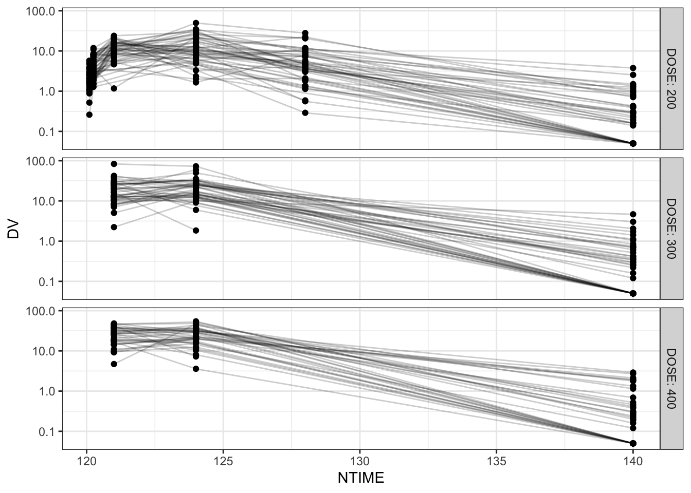
There are three dose group: the lower dose group 200 has relatively intensive sampling, and the higher dose group has relatively sparse sampling. Let’s check the number of subjects per dose group.
data %>% distinct(ID, .keep_all=TRUE) %>% count(DOSE) DOSE n
1 200 50
2 300 50
3 400 50model is developed based on data. We’d like to evaluate model performance, so we plan to simulate from model, and then visually compare the simulations with the observations (i.e., data).
Let’s start simple with 200 mg dose group only.
# Subset
data_200 <- filter(data, DOSE==200)

# Simulation 1 (Single simulation)
inventory(mod, data)

withr::with_seed(
  seed=123,
  sim <- mrgsim_df(mod, data_200, obsonly=TRUE, recover="DV,NTIME,DOSE")
  )
Compare simulation with observations?
obs <- data_200 %>% filter(EVID==0)

p1 <- raw_pk_plot(obs)+ggtitle("Observed")+scale_y_log10(limits = c(0.0001, 1000))
p2 <- raw_pk_plot(sim, .y=Y)+ggtitle("Simulated")+scale_y_log10(limits = c(0.0001, 1000))
grid.arrange(p1, p2, ncol=2)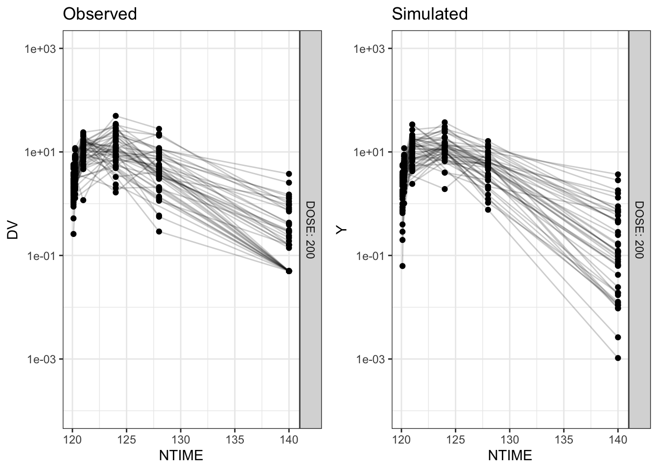
Are the simulated and observed PK profiles look similar enough? Maybe not so easy to tell? Let’s look at it in another way…
# Another way to compare
p3 <- sim %>% group_by(NTIME, DOSE) %>%
    summarise(
      as_tibble_row(
        quantile(Y, c(0.025, 0.500, 0.975),na.rm = TRUE),
        .name_repair= ~ c("lo", "mi", "hi")
      ),
      .groups = "drop") %>%
  ggplot(aes(x=NTIME))+
    geom_line(aes(y=mi))+
    geom_ribbon(aes(ymin=lo, ymax=hi), alpha=0.25)+
    facet_grid(vars(DOSE), labeller=label_both)+
  scale_y_log10()+
  ggtitle("Simulated")+
  ylab("Y")

grid.arrange(p1, p3, ncol=2)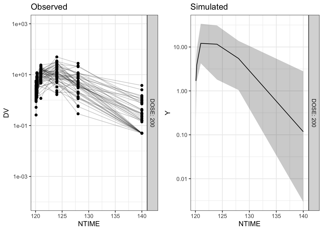
rm(p1,p2,p3) # Remove figure outputs to save RAMOr more commonly…
#' the codes to generate the above plots have been wrapped in `summ_pk_plot()` function
p1 <- summ_pk_plot(sim, .y=Y, show_obs=TRUE)
p1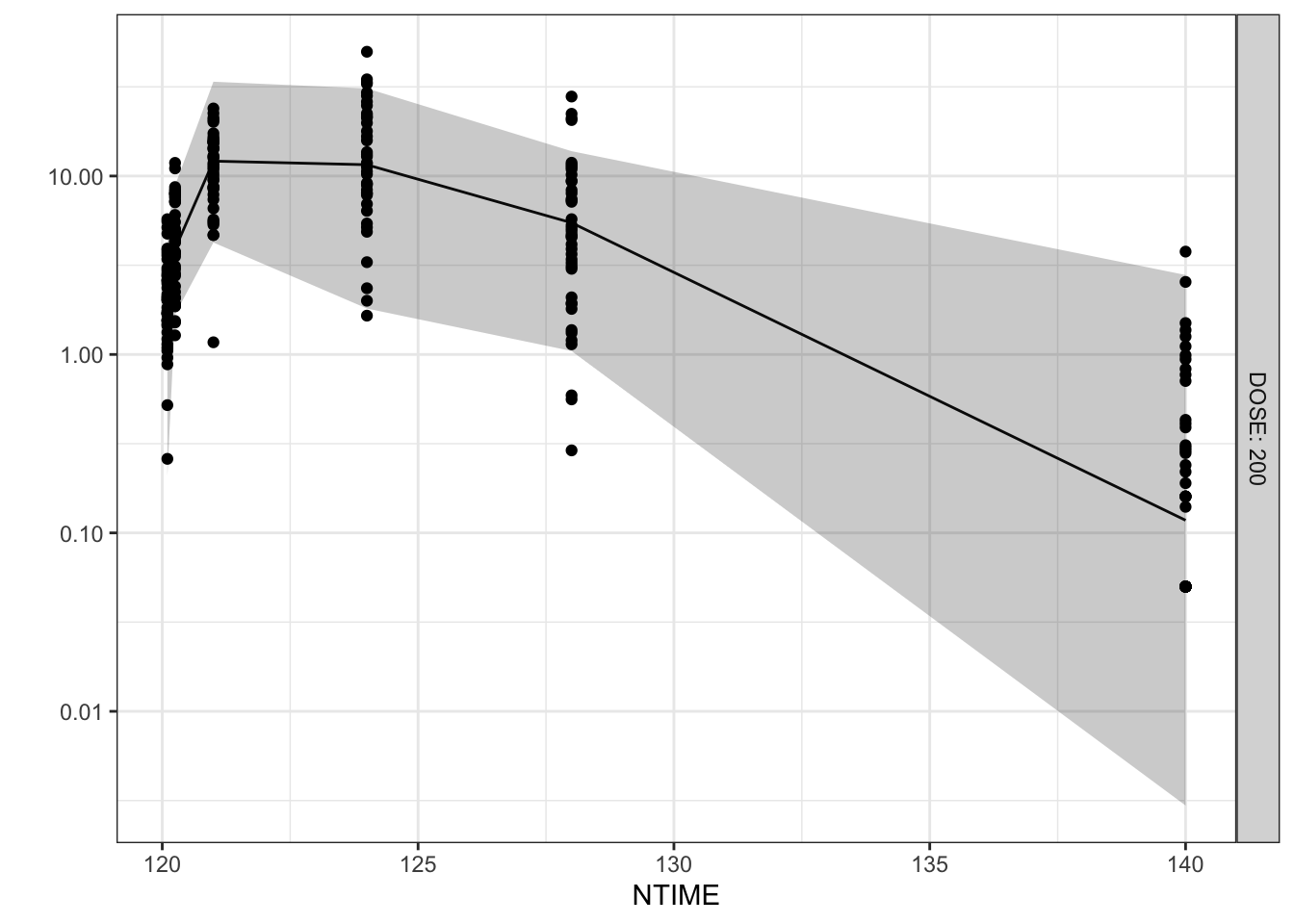
However, we may not reply on one stochastic simulation to evaluate the model performance. If we simulate using the same settings for a second time, it will look different compared to the first simulation.
withr::with_seed(
  seed=321,
  sim2 <- mrgsim_df(mod, data_200, obsonly=TRUE, recover="DV,NTIME,DOSE")
  )
p2 <- summ_pk_plot(sim2, .y=Y, show_obs=TRUE)
grid.arrange(p1, p2, ncol=2)
rm(p1, p2, sim, sim2) # Remove figure outputs to save RAMTherefore, we need to simulate with replicates (e.g., n=100) to evaluate the totality of the stochastic simulations.
rep <- 100

withr::with_seed(seed=1314,
                 sim <- purrr::map(1:rep, function(.irep){
                   mrgsim_df(mod, data_200, obsonly=TRUE, recover="DV,NTIME,DOSE") %>%
                  mutate(IREP=.irep)
                   }) %>% bind_rows()
                 )
…But then how we should effectively visualize it?
p1 <- sim %>% filter(IREP<10) %>%
  summ_pk_plot(., .y=Y, show_obs=TRUE)+
  facet_wrap(~IREP)
p1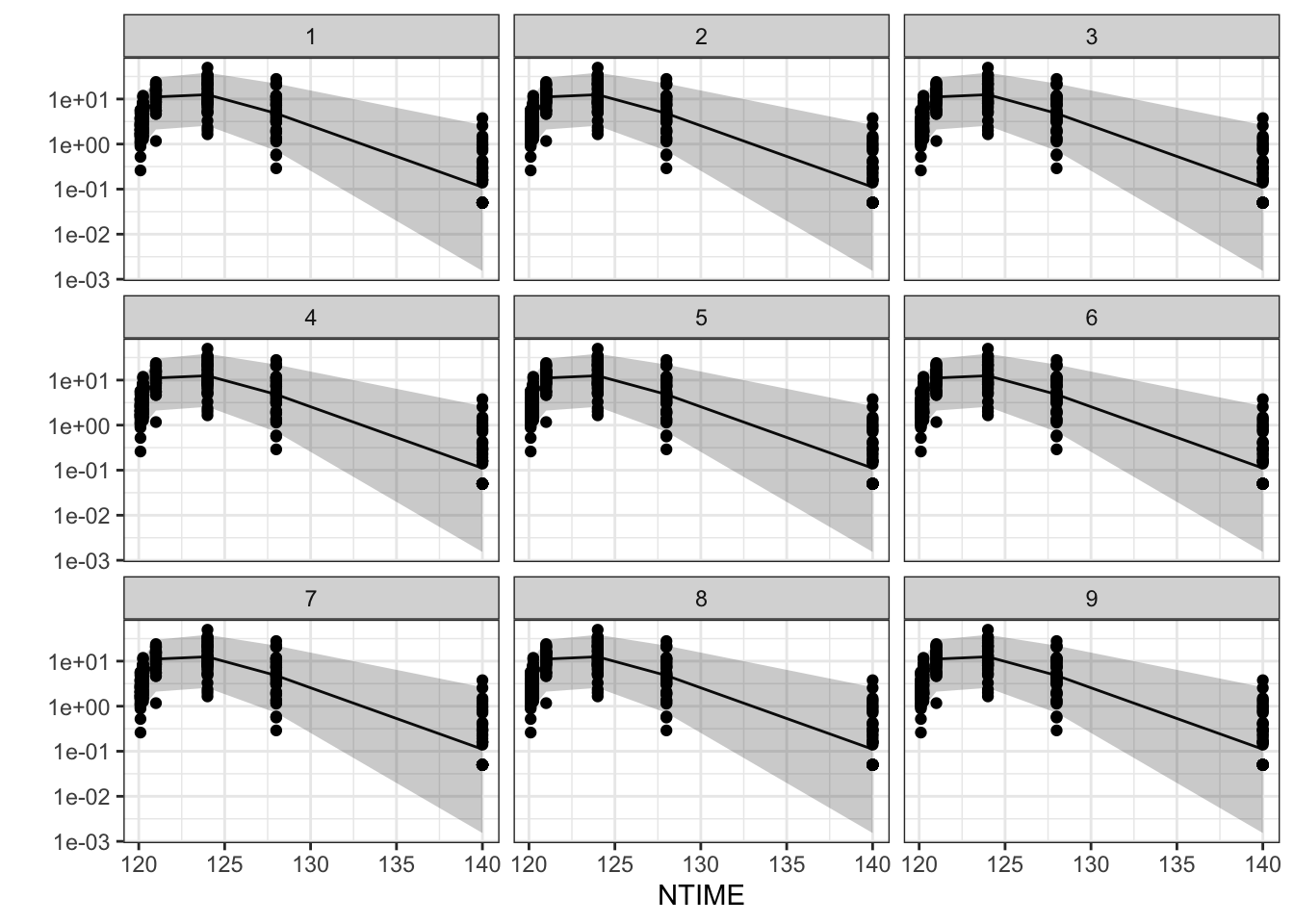
rm(p1) # Remove figure outputs to save RAMGoing through 100 (or more) observation versus simulation plots to determine the proportion showing adequate predictive performance is impractical and inefficient. A more systematic and informative visualization strategy is therefore needed.
VPC was created as an effective way to visualize simulation versus prediction for the evaluation of model predictive performance:
For observed PK profiles, we will summarize:
10th percentile.
50th percentile.
90th percentile.
For simulated PK profiles, we will summarize:
10th percentile of 10th percentiles across simulation replicates.
50th percentile of 10th percentiles across simulation replicates.
90th percentile of 10th percentiles across simulation replicates.
10th percentile of 50th percentiles across simulation replicates.
50th percentile of 50th percentiles across simulation replicates.
90th percentile of 50th percentiles across simulation replicates.
10th percentile of 90th percentiles across simulation replicates.
50th percentile of 90th percentiles across simulation replicates.
90th percentile of 90th percentiles across simulation replicates.
percentile <- c(0.10, 0.50, 0.90) # Percentiles for visualization
prob       <- c(0.10, 0.50, 0.90) # %PI for percentiles

# Summarise observed percentiles
summ_obs <- obs %>%
  filter(BLQ==0) %>%
  group_by(NTIME, DOSE) %>%
  summarise(
    as_tibble_row(
      quantile(DV, percentile,na.rm = TRUE),
      .name_repair= ~ c("lo", "mi", "hi")
      ), .groups = "drop")

# Summarise simulated percentiles
summ_sim <- sim %>%  filter(Y>=unique(obs$LLOQ)) %>%
  group_by(NTIME, DOSE, IREP) %>%
    summarise(
      as_tibble_row(
        quantile(Y, percentile,na.rm = TRUE),
        .name_repair= ~ c("lo", "mi", "hi")
      ), .groups = "drop")

# Summarise prediction intervals of simulated percentiles
summ_sim <- summ_sim %>% group_by(NTIME, DOSE) %>%
  summarise(
    across(c("lo", "mi", "hi"),
           ~ list(setNames(
             quantile(.x, prob, na.rm = TRUE),
             c("lo", "mi", "hi")
             ))), .groups = "drop") %>%
    # widen each list-column (one per Y) into 3 numeric columns
unnest_wider(c("lo", "mi", "hi"), names_sep = "_")head(obs) C NUM ID TIME NTIME TAD AMT CMT EVID II ADDL DV BLQ LLOQ DOSE AGE SEX
1 . 2 51 120.09 120.1 0.09 0 2 0 0 0 5.57 0 0.1 200 18 2
2 . 3 51 121.04 121.0 1.04 0 2 0 0 0 15.43 0 0.1 200 18 2
3 . 4 51 124.07 124.0 4.07 0 2 0 0 0 33.57 0 0.1 200 18 2
4 . 5 51 128.24 128.0 8.24 0 2 0 0 0 20.59 0 0.1 200 18 2
5 . 6 51 139.22 140.0 19.22 0 2 0 0 0 0.99 0 0.1 200 18 2
6 . 8 52 120.10 120.1 0.10 0 2 0 0 0 3.59 0 0.1 200 80 2
RACE ALB SCR WT HT
1 3 4.4 0.72 56.9 160.7
2 3 4.4 0.72 56.9 160.7
3 3 4.4 0.72 56.9 160.7
4 3 4.4 0.72 56.9 160.7
5 3 4.4 0.72 56.9 160.7
6 3 4.3 0.92 78.2 152.6head(sim) ID TIME depot cent CL V IPRED Y
1 51 120.09 191.20067113 10.856582 0.5806127 2.746617 3.952711 6.314298
2 51 121.04 118.90484013 73.862778 0.5806127 2.746617 26.892279 49.059142
3 51 124.07 26.13625703 102.211776 0.5806127 2.746617 37.213704 53.617478
4 51 128.24 3.24892283 55.456425 0.5806127 2.746617 20.190814 17.131533
5 51 139.22 0.01341105 5.973308 0.5806127 2.746617 2.174788 4.061090
6 52 120.10 190.24705382 9.503972 1.9144245 3.564264 2.666461 2.674427
DV NTIME DOSE IREP
1 5.57 120.1 200 1
2 15.43 121.0 200 1
3 33.57 124.0 200 1
4 20.59 128.0 200 1
5 0.99 140.0 200 1
6 3.59 120.1 200 1Then we can visualize it in a constructive way, via overlaying observed percentiles against the correspondingly simulated percentiles.
vpc <- ggplot()+
    geom_line(data=summ_obs, aes(x=NTIME, y=lo), linetype=2)+
    geom_line(data=summ_obs, aes(x=NTIME, y=mi), linetype=1)+
    geom_line(data=summ_obs, aes(x=NTIME, y=hi), linetype=2)+
    geom_ribbon(data=summ_sim, aes(x=NTIME, ymin=lo_lo, ymax=lo_hi), alpha=0.25, fill="#ffcc33")+
    geom_ribbon(data=summ_sim, aes(x=NTIME, ymin=mi_lo, ymax=mi_hi), alpha=0.25, fill="#7A0019")+
    geom_ribbon(data=summ_sim, aes(x=NTIME, ymin=hi_lo, ymax=hi_hi), alpha=0.25, fill="#ffcc33")+
    facet_grid(vars(DOSE), labeller=label_both)+
  scale_y_log10()+
  xlab("Time")+
  ylab("Concentrations")+
  ggtitle("Visual Predictive Checks (VPC)")
vpc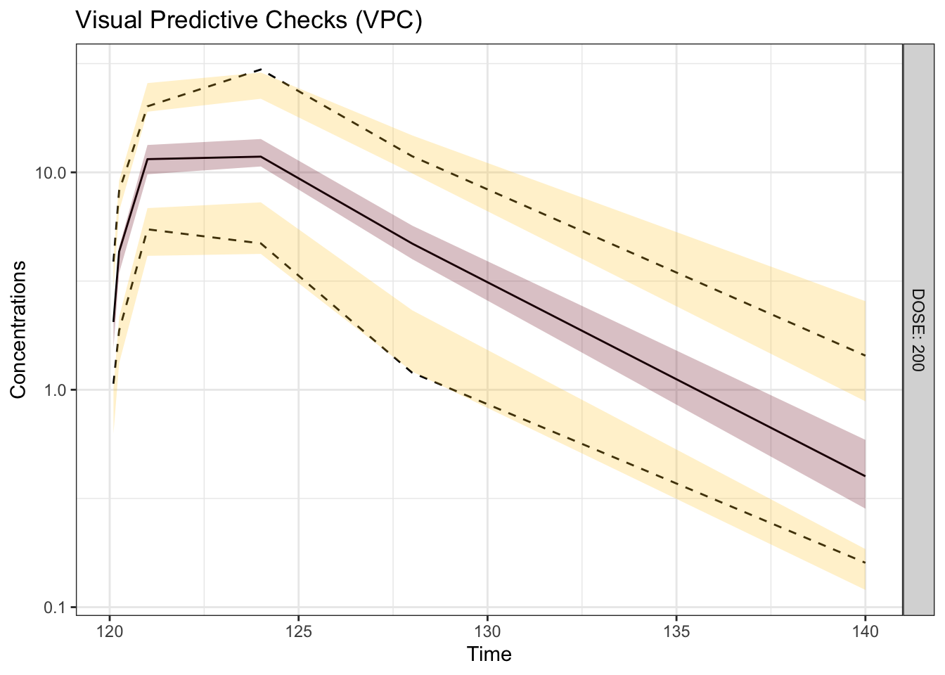
We frequently see VPCs with observed concentrations shown as dots, but this is not something required for diagnostic purposes.
vpc + geom_point(data=filter(obs, BLQ==0), aes(x=NTIME, y=DV))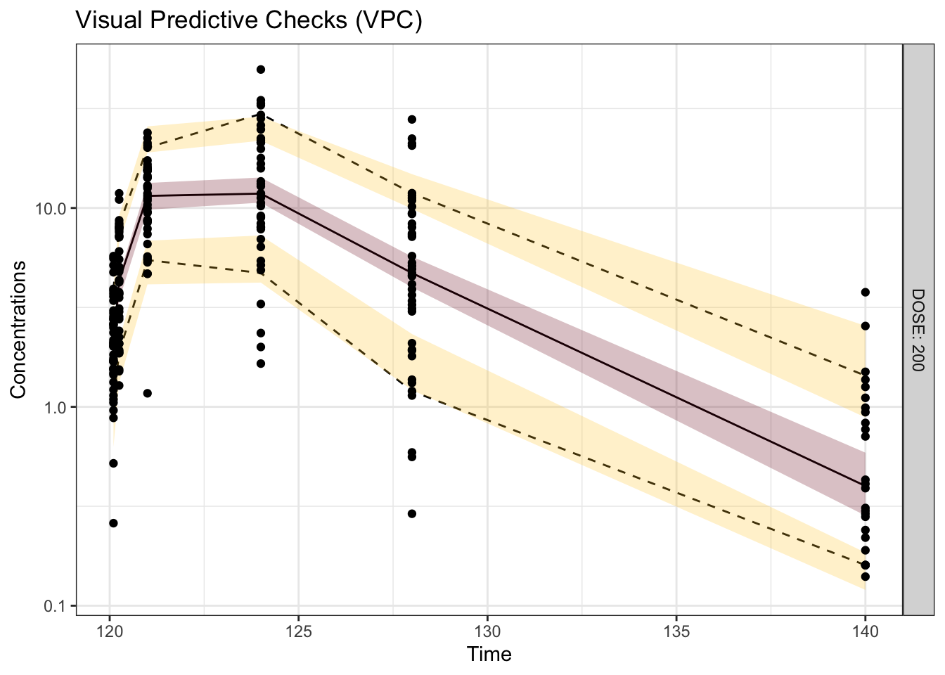
From now on, I will use vpcplot() helper function for the generation of VPCs to prevent repetitive coding.
vpcplot(obs_df=filter(obs, BLQ==0),
        sim_df=filter(sim, Y>unique(obs$LLOQ)),
        show_obs = TRUE, .xlab = "Time", .ylab = "Concentrations")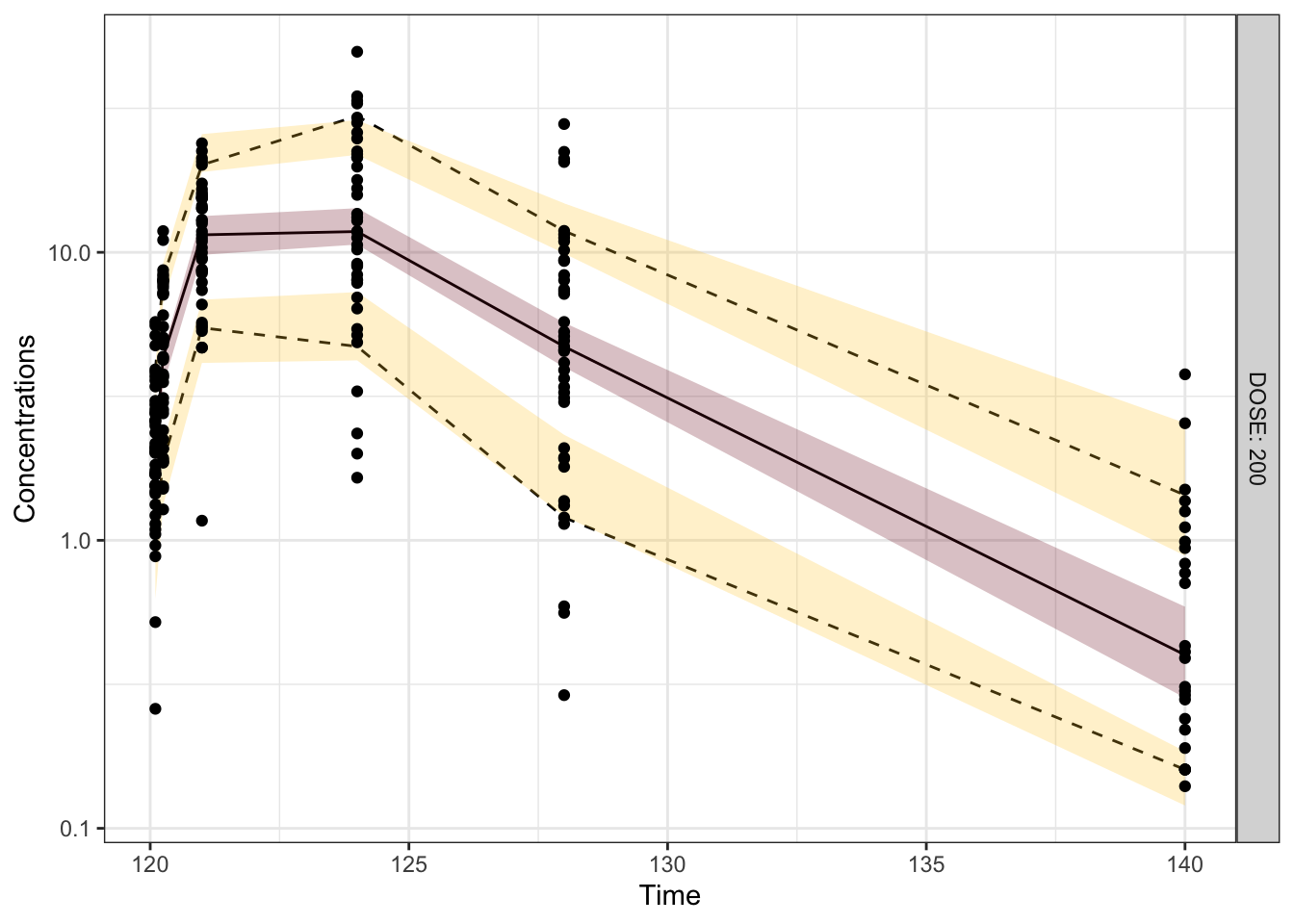
On a separate note, we can also construct VPCs for proportion of observations below LLOQ using a similar approach.
# Summarise observed percentiles
summ_obs2 <- obs %>%
  group_by(NTIME, DOSE) %>%
  summarise(prop = sum(BLQ)/n(), .groups = "drop")

# Summarise simulated percentiles
summ_sim2 <- sim %>%
  group_by(NTIME, DOSE, IREP) %>%
  summarise(prop = sum(Y < unique(obs$LLOQ))/n(), .groups = "drop")

# Summarise prediction intervals of simulated percentiles
summ_sim2 <- summ_sim2 %>% group_by(NTIME, DOSE) %>%
  summarise(
      as_tibble_row(
        quantile(prop, c(0.025, 0.5, 0.975),na.rm = TRUE),
        .name_repair= ~ c("lo", "mi", "hi")
      ), .groups = "drop")

# VPC plot
vpc2 <- ggplot()+
    geom_line(data=summ_obs2, aes(x=NTIME, y=prop), linetype=2)+
    geom_ribbon(data=summ_sim2, aes(x=NTIME, ymin=lo, ymax=hi), alpha=0.25, fill="#7A0019")+
    facet_grid(vars(DOSE), labeller=label_both)+
  xlab("Time")+
  ylab("Proportion of concentrations below LLOQ")+
  ggtitle("Visual Predictive Checks (VPC) for Left Censoring")
vpc2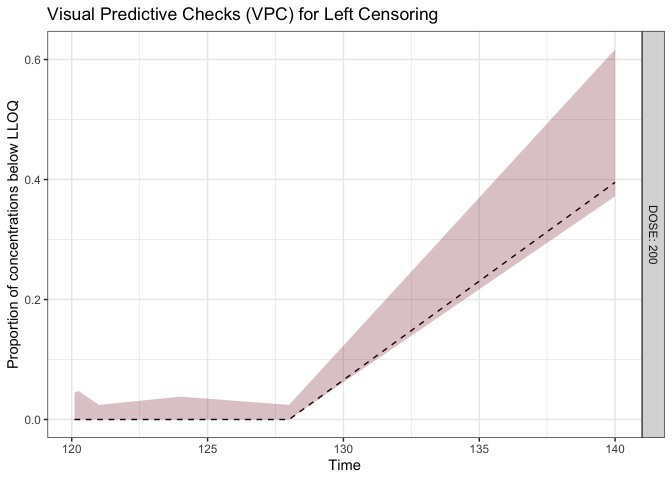
If you have worked on creating VPCs before, an tedious (or somewhat annoying) issue is binning. Why bothering with it?
In reality, we usually develop model using actual time instead of nominal time.
This makes the summarization of the percentiles across time become challenging.
p1  <- raw_pk_plot(obs, .x=NTIME)+ggtitle("Nominal time")
p2  <- raw_pk_plot(obs, .x=TIME)+ggtitle("Actual time")
p3 <- vpcplot(obs_df=filter(obs, BLQ==0),
              sim_df=filter(sim, Y>unique(obs$LLOQ)),
              .x=NTIME, show_obs = TRUE, .xlab = "Time", .ylab = "Concentrations")+
  ggtitle("VPC using nominal time")
p4 <- vpcplot(obs_df=filter(obs, BLQ==0),
              sim_df=filter(sim, Y>unique(obs$LLOQ)),
              .x=TIME, show_obs = TRUE, .xlab = "Time", .ylab = "Concentrations")+
  ggtitle("VPC using actual time")
grid.arrange(p1,p2,p3,p4,ncol=2)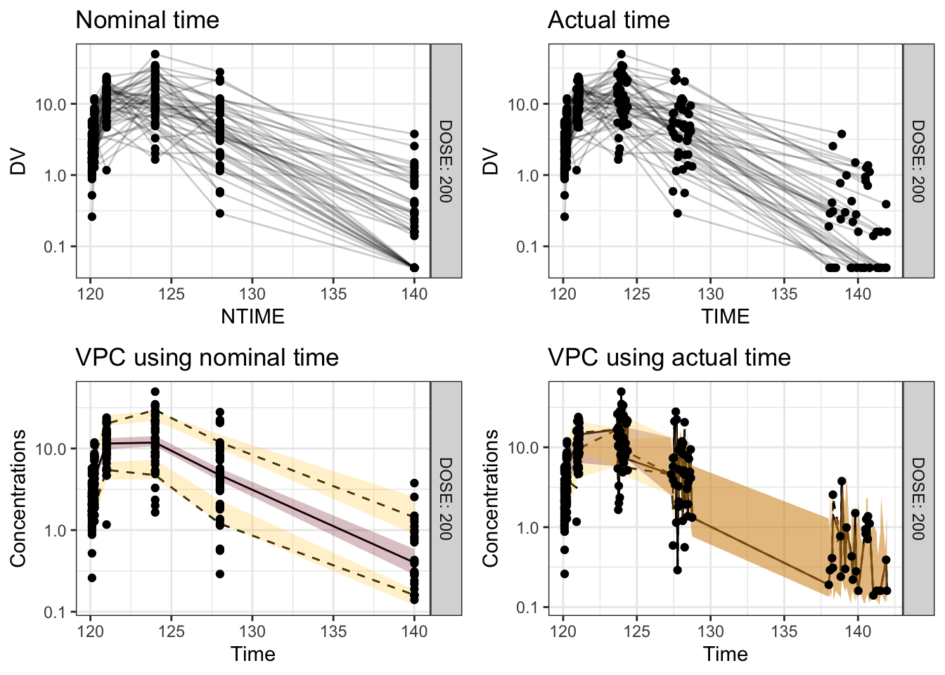
rm(p1, p2, p3, p4) # Remove figure outputs to save RAMAs you can tell, as we created VPCs using actual time without binning, the plot (bottom right) looks messy, losing diagnostic values. This is why we want to bin observations based on time intervals when creating VPCs plots. Essentially, this step classifies actual time into time intervals/bins (i.e., binning), and then summarize observations via grouping by time bins instead of actual times.
This step is illustrated as a multi-step process below:
.bin)bins <- c(119, 120.15, 120.5, 122, 126, 130, 150)
bins <- sort(unique(as.numeric(bins)))
ticks <- cut(bins, breaks = bins)[-1]
mids <- (bins[-1] + bins[-length(bins)]) / 2 # Calculate midpoints for plotting
fobs <- obs %>% mutate(
.bin = cut(TIME, breaks = bins, include.lowest = TRUE, right = TRUE),
.x_plot = mids[as.integer(.bin)]) %>%
dplyr::select(C, NUM, ID, TIME, .bin, .x_plot, NTIME, everything())
fsim <- sim %>% mutate(
.bin = cut(TIME, breaks = bins, include.lowest = TRUE, right = TRUE),
.x_plot = mids[as.integer(.bin)]) %>%
dplyr::select(ID, TIME, .bin, .x_plot, everything()).bin created in step 5.1, instead of NTIMEpercentile <- c(0.10, 0.50, 0.90) # Percentiles for visualization
prob <- c(0.10, 0.50, 0.90) # %PI for percentiles
# Summarise observed percentiles
summ_obs <- fobs %>%
filter(BLQ==0) %>%
group_by(.x_plot, DOSE) %>%
summarise(
as_tibble_row(
quantile(DV, percentile,na.rm = TRUE),
.name_repair= ~ c("lo", "mi", "hi")
), .groups = "drop")
# Summarise simulated percentiles
summ_sim <- fsim %>%
filter(Y > unique(fobs$LLOQ)) %>%
group_by(.x_plot, DOSE, IREP) %>%
summarise(
as_tibble_row(
quantile(Y, percentile,na.rm = TRUE),
.name_repair= ~ c("lo", "mi", "hi")
), .groups = "drop")
# Summarise prediction intervals of simulated percentiles
summ_sim <- summ_sim %>% group_by(.x_plot, DOSE) %>%
summarise(
across(c("lo", "mi", "hi"),
~ list(setNames(
quantile(.x, prob, na.rm = TRUE),
c("lo", "mi", "hi")
))), .groups = "drop") %>%
# widen each list-column (one per Y) into 3 numeric columns
unnest_wider(c("lo", "mi", "hi"), names_sep = "_")vpc <- ggplot()+
geom_line(data=summ_obs, aes(x=.x_plot, y=lo), linetype=2)+
geom_line(data=summ_obs, aes(x=.x_plot, y=mi), linetype=1)+
geom_line(data=summ_obs, aes(x=.x_plot, y=hi), linetype=2)+
geom_ribbon(data=summ_sim, aes(x=.x_plot, ymin=lo_lo, ymax=lo_hi), alpha=0.25, fill="#ffcc33")+
geom_ribbon(data=summ_sim, aes(x=.x_plot, ymin=mi_lo, ymax=mi_hi), alpha=0.25, fill="#7A0019")+
geom_ribbon(data=summ_sim, aes(x=.x_plot, ymin=hi_lo, ymax=hi_hi), alpha=0.25, fill="#ffcc33")+
geom_point(data=filter(obs, BLQ==0), aes(x=TIME, y=DV))+
facet_grid(vars(DOSE), labeller=label_both)+
scale_y_log10()+
xlab("Time")+
ylab("Concentrations")+
ggtitle("Visual Predictive Checks (VPC)")+
scale_x_continuous(
limits = range(bins),
expand = expansion(mult = c(0, 0.02)),
sec.axis = dup_axis(
name = NULL,
breaks = bins, # tick positions on top
labels = rep("", length(bins)) # no labels, ticks only
)) + theme(
axis.ticks.x.top = element_line(),
axis.ticks.length.x.top = unit(5, "pt")
)
vpc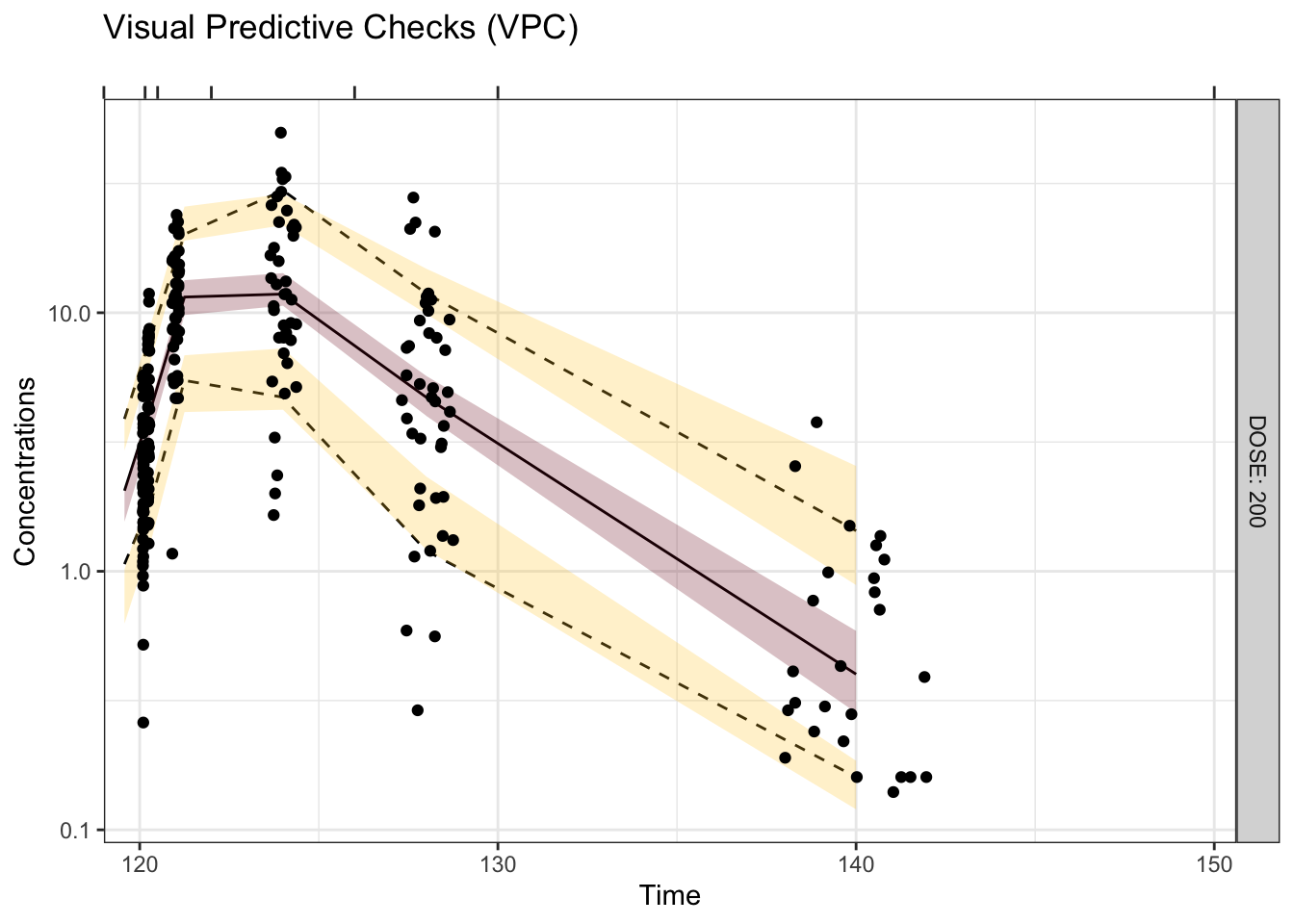
Again, the above process can be wrapped in the helper function to save some codings.
vpcplot(obs_df=filter(obs, BLQ==0),
        sim_df=filter(sim, Y>unique(obs$LLOQ)),
        .x=TIME, show_obs = TRUE,
        .xlab = "Time", .ylab = "Concentrations",
        bins = c(119, 120.15, 120.5, 122, 126, 130, 150))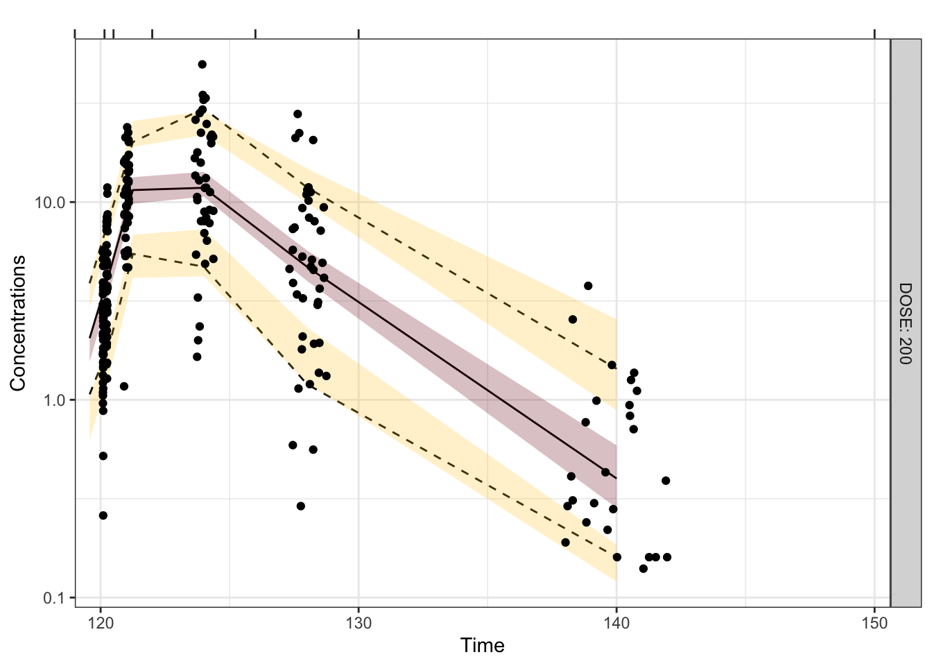
In the presence of influential covariates (e.g., doses), prediction-corrected VPCs (pcVPCs) overcome the challenges when binning across influential covariates with large variability
To illustate this, instead of simulate and evaluate model performance in 200 mg dose group only, let’s simulate and evaluate across multiple dose groups (i.e., 200-400 mg) with diverse sampling scheme (i.e., intensive vs sparse).
rep <- 100
withr::with_seed(seed=4231,
                 sim <- purrr::map(1:rep, function(.irep){
                   mrgsim_df(mod, data, obsonly=TRUE, recover="DV,NTIME,DOSE") %>%
                     mutate(IREP=.irep)
                   }) %>% bind_rows()
                 )

obs <- data %>% filter(EVID==0)

vpc <- vpcplot(obs_df=filter(obs, BLQ==0),
               sim_df=filter(sim, Y>unique(obs$LLOQ)),
               .x=TIME, show_obs = TRUE,
               .facet = NULL, .color = DOSE, .xlab = "Time", .ylab="Concentrations",
               bins = c(119, 120.15, 120.5, 122, 126, 130, 150))+
  ggtitle("VPCs")+
  theme(legend.position = "bottom")
vpc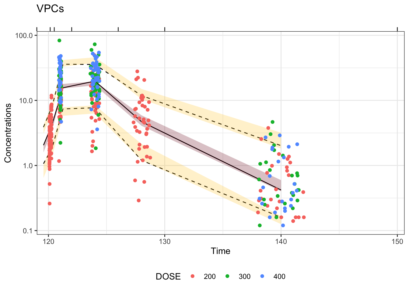
VPCs created via binning across influential covariates (e.g., dose) may compromise the diagnostic values (M. Bergstrand, et al., AAPS J 2011. One way to overcome this is to stratify by the covariates or create VPCs using transformed observations(e.g., dose normalized observations).
# Multiple doses
vpcplot(obs_df=filter(obs, BLQ==0),
        sim_df=filter(sim, Y>unique(obs$LLOQ)),
        .x=TIME, show_obs = TRUE,
        bins = c(119, 120.15, 120.5, 122, 126, 130, 150))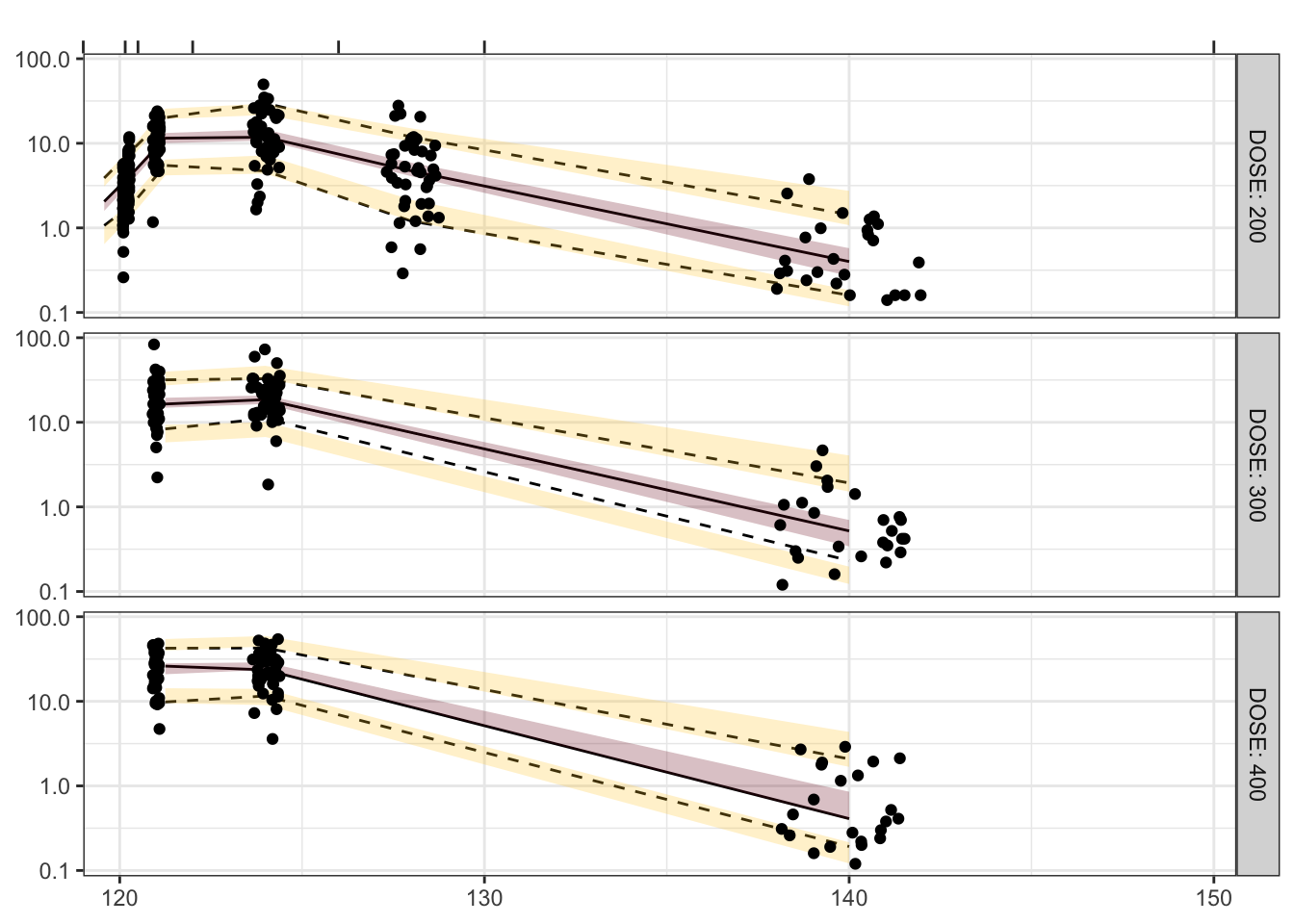
While it occasionally works well (like the example shown above), this does not always work as expected since some subgroups may have very sparse data, inadequate for percentile summarizations and further VPC creations. Dose normalizations may be complicated due to dose modifications or interruptions. In these situations, prediction-corrected VPCs (pcVPCs) can be useful to address these issues.
Population predictions (PRED) are needed (for normalization purpose) to create pcVPCs. This is commonly output by modeling software (e.g., NONMEM). In our case, we simulate PRED by zero-out random effects.
pred <- mrgsim_df(zero_re(mod), data, outvars="IPRED") %>% rename(PRED=IPRED)
data <- data %>% left_join(pred)
obs <- data %>% filter(EVID==0)
Let’s redo the simulation and carry out PRED for creating pcVPC.
set.seed(4231)
sim <- purrr::map(1:rep, function(.irep){
  mrgsim_df(mod, data, obsonly=TRUE, recover="DV,NTIME,DOSE,PRED") %>%
    mutate(IREP=.irep)
}) %>% bind_rows()
Then repeat the same multi-step process for creating VPCs.
bins <- c(119, 120.15, 120.5, 122, 126, 130, 150)
# bins <- c(119, 120.15, 120.5, 122, 124, 126, 130, 150)

bins <- sort(unique(as.numeric(bins)))
ticks <- cut(bins, breaks = bins)[-1]
mids  <- (bins[-1] + bins[-length(bins)]) / 2 # Calculate midpoints for plotting

fobs <- obs %>% mutate(
  .bin = cut(TIME, breaks = bins, include.lowest = TRUE, right = TRUE),
  .x_plot = mids[as.integer(.bin)]) %>%
  dplyr::select(C, NUM, ID, TIME, .bin, .x_plot, NTIME, everything())

fsim <- sim %>% mutate(
  .bin = cut(TIME, breaks = bins, include.lowest = TRUE, right = TRUE),
  .x_plot = mids[as.integer(.bin)]) %>%
dplyr::select(ID, TIME, .bin, .x_plot, everything())PRED normalized observed and simulated outcomes\[ pcY_{ij}=lb_{ij}+(Y_{ij}-lb_{ij}) \times \frac{\widetilde{PRED_{bin}}-lb_{ij}}{PRED_{ij}-lb_{ij}} \\ \]
Assuming an outcome with lower bound of 0 (i.e., \(lb_{ij}=0\)), such as concentrations.
\[ pcY_{ij}=Y_{ij} \times \frac{\widetilde{PRED_{bin}}}{PRED_{ij}} \\ \]
percentile <- c(0.10, 0.50, 0.90) # Percentiles for visualization
prob       <- c(0.10, 0.50, 0.90) # %PI for percentiles

# Summarise observed percentiles
summ_obs <- fobs %>% filter(BLQ==0) %>%
      mutate(.yobs = DV/PRED) %>%
      group_by(.bin, .x_plot) %>%
      mutate(pred_bin = median(PRED)) %>%
      mutate(.yobs = .yobs*pred_bin) %>%
      summarise(
        as_tibble_row(
          quantile(.yobs, percentile, na.rm = TRUE),
          .name_repair= ~ c("lo", "mi", "hi")
        ),
        .groups = "drop")

# Summarise simulated percentiles
summ_sim <- fsim %>% filter(Y>unique(obs$LLOQ)) %>%
      mutate(.ysim = Y/PRED) %>%
      group_by(.bin, .x_plot, IREP) %>%
      mutate(pred_bin = median(PRED)) %>%
      mutate(.ysim = .ysim*pred_bin) %>%
      summarise(
        as_tibble_row(
          quantile(.ysim, percentile, na.rm = TRUE),
          .name_repair= ~ c("lo", "mi", "hi")
        ),
        .groups = "drop")

# Summarise prediction intervals of simulated percentiles
summ_sim <- summ_sim %>% group_by(.x_plot) %>%
  summarise(
    across(c("lo", "mi", "hi"),
           ~ list(setNames(
             quantile(.x, prob, na.rm = TRUE),
             c("lo", "mi", "hi")
             ))), .groups = "drop") %>%
    # widen each list-column (one per Y) into 3 numeric columns
unnest_wider(c("lo", "mi", "hi"), names_sep = "_")obs_v <- fobs %>% filter(BLQ==0) %>%
mutate(.yobs = DV/PRED) %>%
group_by(.bin, .x_plot) %>%
mutate(pred_bin = median(PRED)) %>%
mutate(.yobs = .yobs*pred_bin)
pcvpc <- ggplot()+
geom_line(data=summ_obs, aes(x=.x_plot, y=lo), linetype=2)+
geom_line(data=summ_obs, aes(x=.x_plot, y=mi), linetype=1)+
geom_line(data=summ_obs, aes(x=.x_plot, y=hi), linetype=2)+
geom_ribbon(data=summ_sim, aes(x=.x_plot, ymin=lo_lo, ymax=lo_hi), alpha=0.25, fill="#ffcc33")+
geom_ribbon(data=summ_sim, aes(x=.x_plot, ymin=mi_lo, ymax=mi_hi), alpha=0.25, fill="#7A0019")+
geom_ribbon(data=summ_sim, aes(x=.x_plot, ymin=hi_lo, ymax=hi_hi), alpha=0.25, fill="#ffcc33")+
geom_point(data=obs_v, aes(x=TIME, y=.yobs, color=DOSE))+
scale_y_log10()+
xlab("Time")+
ylab("Concentrations")+
ggtitle("pcVPC")+
scale_x_continuous(
limits = range(bins),
expand = expansion(mult = c(0, 0.02)),
sec.axis = dup_axis(
name = NULL,
breaks = bins, # tick positions on top
labels = rep("", length(bins)) # no labels, ticks only
)) + theme(
axis.ticks.x.top = element_line(),
axis.ticks.length.x.top = unit(5, "pt"),
legend.position = "bottom"
)
pcvpc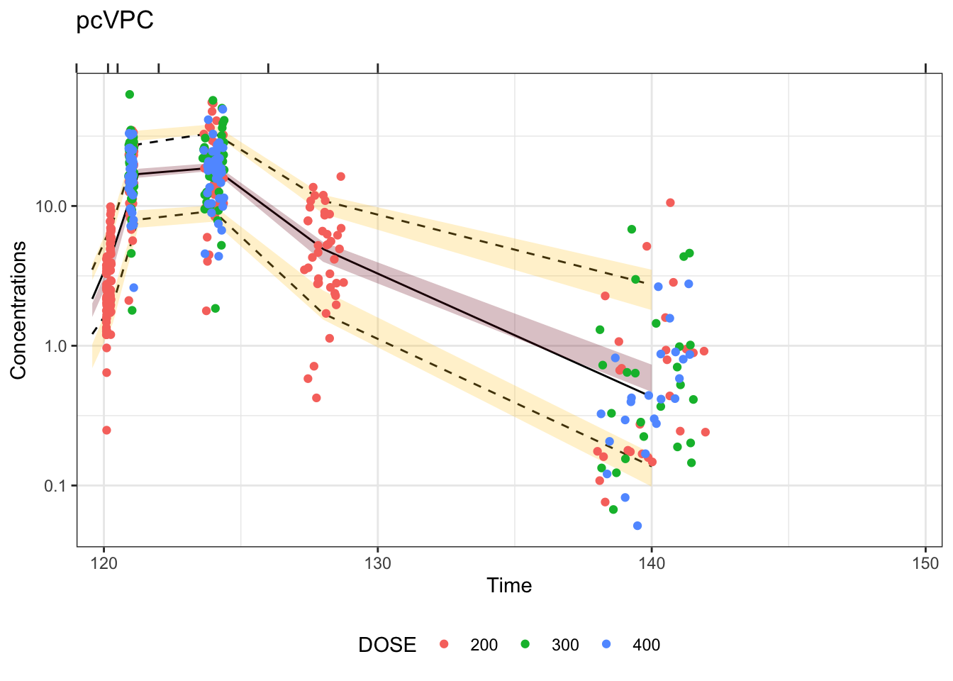
Compare VPC and pcVPC side by side.
vpc   <- vpc+scale_y_log10(limits=c(0.01, 200))
pcvpc <- pcvpc+scale_y_log10(limits=c(0.01, 200))

grid.arrange(vpc, pcvpc, ncol=2)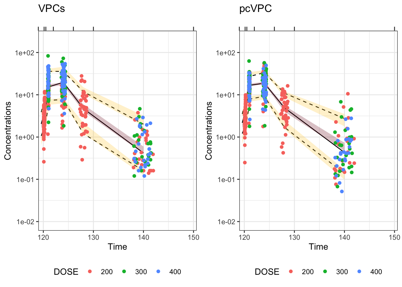
An updated method of VPCs is reference correted VPCs (rcVPCs).
Reference: M. Ibrahim, et al., AAPS J 2025
Unlike pcVPC which normalizes observed and simulated values using median PRED of a bin, rcVPC normalizes observed and simulated values using simulated PRED with reference covariates before binning.
rcVPC provides a more intuitive method for visual model diagnostics.
Note: for this illustration, we didn’t apply variability correction. The original paper did mention variability-correction is recommended and is applied by default if using PsN program.
First, let’s again redo the simulation and carry out PRED for creating rcVPC.
set.seed(4231)
obs <- data %>% filter(EVID==0)
sim <- purrr::map(1:rep, function(.irep){
  mrgsim_df(mod, data, obsonly=TRUE, recover="DV,NTIME,DOSE,PRED") %>%
    mutate(IREP=.irep)
}) %>% bind_rows()head(obs) C NUM ID TIME NTIME TAD AMT CMT EVID II ADDL DV BLQ LLOQ DOSE AGE SEX
1 . 2 51 120.09 120.1 0.09 0 2 0 0 0 5.57 0 0.1 200 18 2
2 . 3 51 121.04 121.0 1.04 0 2 0 0 0 15.43 0 0.1 200 18 2
3 . 4 51 124.07 124.0 4.07 0 2 0 0 0 33.57 0 0.1 200 18 2
4 . 5 51 128.24 128.0 8.24 0 2 0 0 0 20.59 0 0.1 200 18 2
5 . 6 51 139.22 140.0 19.22 0 2 0 0 0 0.99 0 0.1 200 18 2
6 . 8 52 120.10 120.1 0.10 0 2 0 0 0 3.59 0 0.1 200 80 2
RACE ALB SCR WT HT PRED
1 3 4.4 0.72 56.9 160.7 2.527803
2 3 4.4 0.72 56.9 160.7 17.906666
3 3 4.4 0.72 56.9 160.7 24.180457
4 3 4.4 0.72 56.9 160.7 12.509704
5 3 4.4 0.72 56.9 160.7 1.154850
6 3 4.3 0.92 78.2 152.6 1.713551head(sim) ID TIME depot cent CL V IPRED Y DV
1 51 120.09 191.20067114 9.381783 1.950703 7.301553 1.2849025 1.242802 5.57
2 51 121.04 118.90484010 70.492336 1.950703 7.301553 9.6544306 10.633398 15.43
3 51 124.07 26.13625703 88.895122 1.950703 7.301553 12.1748240 9.569857 33.57
4 51 128.24 3.24892283 40.622005 1.950703 7.301553 5.5634748 4.085091 20.59
5 51 139.22 0.01341105 2.504090 1.950703 7.301553 0.3429531 0.362332 0.99
6 52 120.10 190.24705382 9.429376 3.106647 4.554514 2.0703367 2.083674 3.59
NTIME DOSE PRED IREP
1 120.1 200 2.527803 1
2 121.0 200 17.906666 1
3 124.0 200 24.180457 1
4 128.0 200 12.509704 1
5 140.0 200 1.154850 1
6 120.1 200 1.713551 1Simulate reference population predictions (PREDREF) based on arbitrarily selected reference covariates:
Dose=300.
WT=70.
AGE=35.
ALB=4.5.
SEX=1
data_ref <- data %>%
  dplyr::select(-all_of(c("DOSE", "AGE", "SEX", "RACE",
                          "ALB" , "SCR", "WT" , "HT"))) %>%
  mutate(AMT = ifelse(AMT != 0, 300, AMT))

param_tags(mod)
name tag
1 WT input
2 SEX input
3 AGE input
4 ALB inputrep <- 100
sim_ref <- mrgsim_df(zero_re(mod), data_ref, outvars="IPRED", obsonly=TRUE) %>% rename(PREDREF=IPRED)
head(sim_ref) ID TIME PREDREF
1 51 120.09 2.712769
2 51 121.04 20.700633
3 51 124.07 24.671124
4 51 128.24 10.235147
5 51 139.22 0.460132
6 52 120.10 2.990299\[ rcY_{ij}^*=lb_{ij}+(Y_{ij}-lb_{ij}) \times \frac{PRED_{ij,ref}-lb_{ij}}{PRED_{ij}-lb_{ij}} \\ \]
Assuming an outcome with lower bound of 0 (i.e., \(lb_{ij}=0\)), such as concentrations.
\[ rcY_{ij}^*=Y_{ij} \times \frac{PRED_{ij,ref}}{PRED_{ij}} \\ \]
obs_with_ref <- left_join(obs, sim_ref) %>%
  mutate(RCDV_HAT = (DV / PRED) * PREDREF) %>%
  dplyr::select(C, NUM, ID, TIME, PRED, PREDREF,
                RCDV_HAT, everything())
Joining with `by = join_by(ID, TIME)`sim_with_ref <- left_join(sim, sim_ref) %>%
mutate(RCY_HAT = (Y / PRED) * PREDREF) %>%
dplyr::select(ID, TIME, PRED, PREDREF,
RCY_HAT, everything())Joining with `by = join_by(ID, TIME)`head(obs_with_ref) C NUM ID TIME PRED PREDREF RCDV_HAT NTIME TAD AMT CMT EVID II
1 . 2 51 120.09 2.527803 2.712769 5.977572 120.1 0.09 0 2 0 0
2 . 3 51 121.04 17.906666 20.700633 17.837535 121.0 1.04 0 2 0 0
3 . 4 51 124.07 24.180457 24.671124 34.251198 124.0 4.07 0 2 0 0
4 . 5 51 128.24 12.509704 10.235147 16.846256 128.0 8.24 0 2 0 0
5 . 6 51 139.22 1.154850 0.460132 0.394450 140.0 19.22 0 2 0 0
6 . 8 52 120.10 1.713551 2.990299 6.264869 120.1 0.10 0 2 0 0
ADDL DV BLQ LLOQ DOSE AGE SEX RACE ALB SCR WT HT
1 0 5.57 0 0.1 200 18 2 3 4.4 0.72 56.9 160.7
2 0 15.43 0 0.1 200 18 2 3 4.4 0.72 56.9 160.7
3 0 33.57 0 0.1 200 18 2 3 4.4 0.72 56.9 160.7
4 0 20.59 0 0.1 200 18 2 3 4.4 0.72 56.9 160.7
5 0 0.99 0 0.1 200 18 2 3 4.4 0.72 56.9 160.7
6 0 3.59 0 0.1 200 80 2 3 4.3 0.92 78.2 152.6head(sim_with_ref) ID TIME PRED PREDREF RCY_HAT depot cent CL
1 51 120.09 2.527803 2.712769 1.3337408 191.20067114 9.381783 1.950703
2 51 121.04 17.906666 20.700633 12.2925218 118.90484010 70.492336 1.950703
3 51 124.07 24.180457 24.671124 9.7640472 26.13625703 88.895122 1.950703
4 51 128.24 12.509704 10.235147 3.3423261 3.24892283 40.622005 1.950703
5 51 139.22 1.154850 0.460132 0.1443655 0.01341105 2.504090 1.950703
6 52 120.10 1.713551 2.990299 3.6361966 190.24705382 9.429376 3.106647
V IPRED Y DV NTIME DOSE IREP
1 7.301553 1.2849025 1.242802 5.57 120.1 200 1
2 7.301553 9.6544306 10.633398 15.43 121.0 200 1
3 7.301553 12.1748240 9.569857 33.57 124.0 200 1
4 7.301553 5.5634748 4.085091 20.59 128.0 200 1
5 7.301553 0.3429531 0.362332 0.99 140.0 200 1
6 4.554514 2.0703367 2.083674 3.59 120.1 200 1bins <- c(119, 120.15, 120.5, 122, 126, 130, 150)
bins <- sort(unique(as.numeric(bins)))
ticks <- cut(bins, breaks = bins)[-1]
mids <- (bins[-1] + bins[-length(bins)]) / 2 # Calculate midpoints for plotting
fobs <- obs_with_ref %>% mutate(
.bin = cut(TIME, breaks = bins, include.lowest = TRUE, right = TRUE),
.x_plot = mids[as.integer(.bin)]) %>%
dplyr::select(C, NUM, ID, TIME, .bin, .x_plot, NTIME, everything())
fsim <- sim_with_ref %>% mutate(
.bin = cut(TIME, breaks = bins, include.lowest = TRUE, right = TRUE),
.x_plot = mids[as.integer(.bin)]) %>%
dplyr::select(ID, TIME, .bin, .x_plot, everything())PRED normalized observed and simulated outcomes# | warning: false
percentile <- c(0.10, 0.50, 0.90) # Percentiles for visualization
prob <- c(0.10, 0.50, 0.90) # %PI for percentiles
# Summarise observed percentiles
summ_obs <- fobs %>% filter(BLQ==0) %>%
group_by(.bin, .x_plot) %>%
summarise(
as_tibble_row(
quantile(RCDV_HAT, percentile, na.rm = TRUE),
.name_repair= ~ c("lo", "mi", "hi")
),
.groups = "drop")
# Summarise simulated percentiles
summ_sim <- fsim %>% filter(Y>unique(obs$LLOQ)) %>%
group_by(.bin, .x_plot, IREP) %>%
summarise(
as_tibble_row(
quantile(RCY_HAT, percentile, na.rm = TRUE),
.name_repair= ~ c("lo", "mi", "hi")
),
.groups = "drop")
# Summarise prediction intervals of simulated percentiles
summ_sim <- summ_sim %>% group_by(.x_plot) %>%
summarise(
across(c("lo", "mi", "hi"),
~ list(setNames(
quantile(.x, prob, na.rm = TRUE),
c("lo", "mi", "hi")
))), .groups = "drop") %>%
# widen each list-column (one per Y) into 3 numeric columns
unnest_wider(c("lo", "mi", "hi"), names_sep = "_")obs_v <- fobs %>% filter(BLQ==0)
rcvpc <- ggplot()+
geom_line(data=summ_obs, aes(x=.x_plot, y=lo), linetype=2)+
geom_line(data=summ_obs, aes(x=.x_plot, y=mi), linetype=1)+
geom_line(data=summ_obs, aes(x=.x_plot, y=hi), linetype=2)+
geom_ribbon(data=summ_sim, aes(x=.x_plot, ymin=lo_lo, ymax=lo_hi), alpha=0.25, fill="#ffcc33")+
geom_ribbon(data=summ_sim, aes(x=.x_plot, ymin=mi_lo, ymax=mi_hi), alpha=0.25, fill="#7A0019")+
geom_ribbon(data=summ_sim, aes(x=.x_plot, ymin=hi_lo, ymax=hi_hi), alpha=0.25, fill="#ffcc33")+
geom_point(data=obs_v, aes(x=TIME, y=RCDV_HAT, color=DOSE))+
scale_y_log10()+
xlab("Time")+
ylab("Concentrations")+
ggtitle("rcVPC")+
scale_x_continuous(
limits = range(bins),
expand = expansion(mult = c(0, 0.02)),
sec.axis = dup_axis(
name = NULL,
breaks = bins, # tick positions on top
labels = rep("", length(bins)) # no labels, ticks only
)) + theme(
axis.ticks.x.top = element_line(),
axis.ticks.length.x.top = unit(5, "pt"),
legend.position = "bottom"
)
rcvpc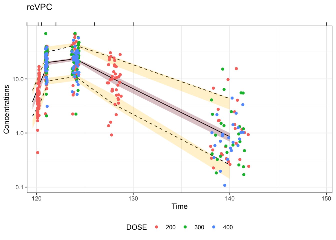
Compare VPC, pcVPC and rcVPC side by side. We can see reference-corrected VPCs have a more natural appearance similar to the shape of the original PK profiles despite the presence of multiple dose groups with different sampling schemes.
rcvpc <- rcvpc + scale_y_log10(limits=c(0.01, 200))Scale for y is already present.
Adding another scale for y, which will replace the existing scale.grid.arrange(vpc, pcvpc, rcvpc, ncol=3)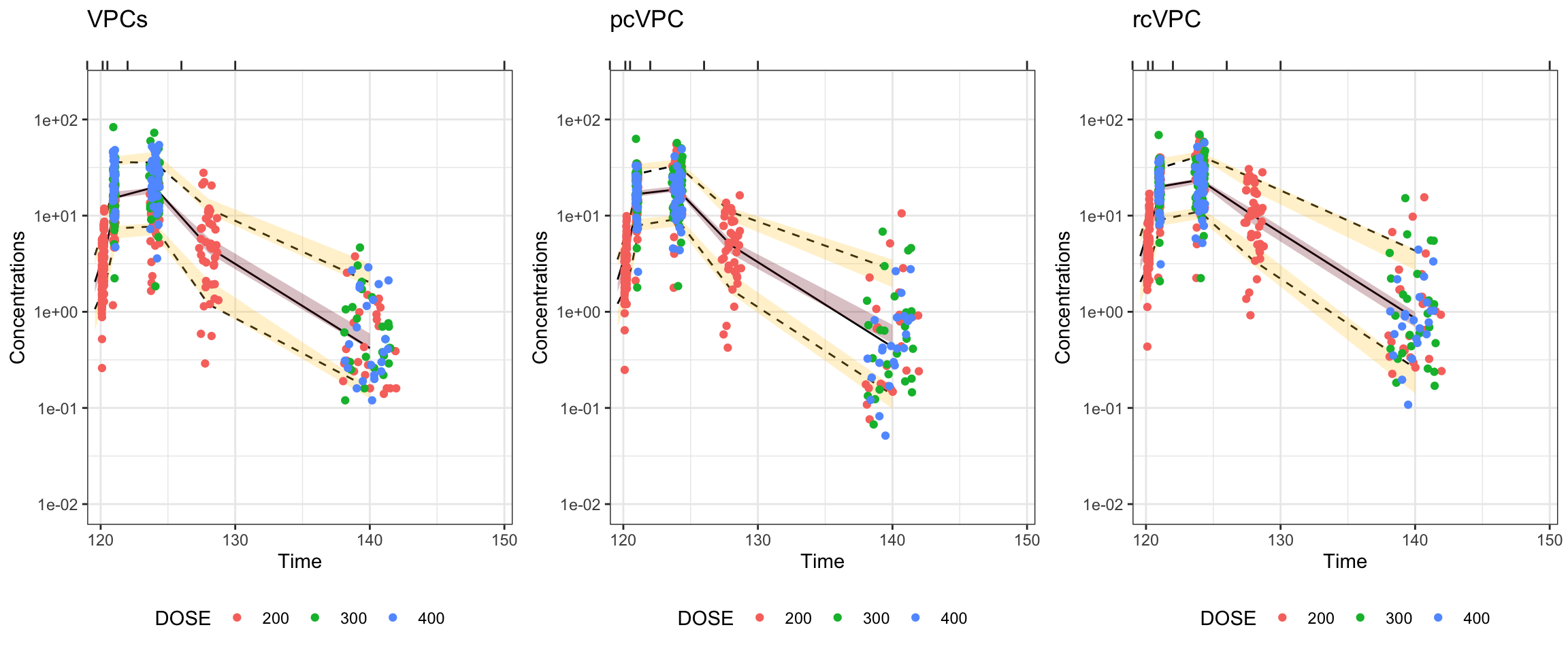
sessionInfo()R version 4.4.3 (2025-02-28)
Platform: x86_64-apple-darwin20
Running under: macOS Sequoia 15.7.3
Matrix products: default
BLAS: /Library/Frameworks/R.framework/Versions/4.4-x86_64/Resources/lib/libRblas.0.dylib
LAPACK: /Library/Frameworks/R.framework/Versions/4.4-x86_64/Resources/lib/libRlapack.dylib; LAPACK version 3.12.0
locale:
[1] en_US.UTF-8/en_US.UTF-8/en_US.UTF-8/C/en_US.UTF-8/en_US.UTF-8
time zone: America/Chicago
tzcode source: internal
attached base packages:
[1] stats graphics grDevices datasets utils methods base
other attached packages:
[1] gridExtra_2.3 mrgsolve_1.7.2 lubridate_1.9.4 forcats_1.0.1
[5] stringr_1.6.0 dplyr_1.1.4 purrr_1.2.1 readr_2.1.6
[9] tidyr_1.3.2 tibble_3.3.1 ggplot2_4.0.1 tidyverse_2.0.0
loaded via a namespace (and not attached):
[1] gtable_0.3.6 jsonlite_1.8.8 compiler_4.4.3 renv_1.1.5
[5] Rcpp_1.1.1 tidyselect_1.2.1 scales_1.4.0 yaml_2.3.8
[9] fastmap_1.1.1 R6_2.5.1 labeling_0.4.3 generics_0.1.4
[13] knitr_1.45 pillar_1.11.1 RColorBrewer_1.1-3 tzdb_0.5.0
[17] rlang_1.1.7 stringi_1.8.7 xfun_0.42 S7_0.2.1
[21] timechange_0.4.0 cli_3.6.2 withr_3.0.2 magrittr_2.0.4
[25] digest_0.6.35 grid_4.4.3 rstudioapi_0.18.0 hms_1.1.4
[29] lifecycle_1.0.4 vctrs_0.7.1 evaluate_0.23 glue_1.7.0
[33] farver_2.1.2 rmarkdown_2.26 tools_4.4.3 pkgconfig_2.0.3
[37] htmltools_0.5.7